“Math – What’s the Use?” by Miller

Introduction:

Behind all great (and not so great) computer graphics images and/or animations stands a great lady. Her name? Mathematics. Whether it is a spline or parametric equations that generate the curve, the various geometries that provide the illusion of 3D, or the vector theory used in reflections, rotations, and shading, just about all aspects of a computer-generated image rely on mathematics. This paper discusses some of the different mathematics used in generating graphics images, from basic Euclidean geometry to the basics of spline interpolation. We begin with an overview of the simpler concepts in computer graphics: line drawing and transformations. In section 2, we examine how the illusion of 3D is created. In section 3, we examine the mathematics involved in lighting our scene. And finally, in section 4, we examine creation of objects that do not have a simple geometric representation.

Section 1: The Basics

Computer graphics techniques have always relied heavily on mathematics for their implementation. Simple line and conic drawing algorithms1,2,3,4 show the importance of a thorough understanding of basic algebra, geometry, and multivariate calculus. Calculus? Yes, gradients are used to determine vectors perpendicular to the tangents to conics other than circles. This is used when determining which pixel to “turn on” to create the most realistic-looking curve. Even pattern filling and line clipping rely on these basic concepts. Then, of course, clipping requires knowledge of the widowing system and coordinate systems in general. So we’re back to geometry again. When creating an object to be represented, a mathematical model representing this object must be created. Whether it is a simple 2D or 3D geometric figure, or a more complicated curve or surface, each object must have a mathematical representation. This representation is given in “real-world” coordinates: real values for which the mathematical model is valid. To create the graphics image to represent our object, we must change the real-world coordinates (window or user coordinates) of our object to the normalized device coordinates and/or the viewport coordinates. This change requires what is commonly referred to as a window-to-viewport transformation. This transformation of user coordinates (xuser ,yuser) to normalized device coordinates (xnorm, ynorm) is a simple linear function that is a combination of scaling and translation:

Here, w_x_min, w_x_max, w_y_min, and w_y_max, are the minimum and maximum window (user) coordinates in the x and y directions, and v_x_min, v_x_max, v_y_min, and v_y_max are the minimum and maximum viewport coordinates in the x and y
directions.

Once we have the ability to represent our object, we may wish to change its position or size or inclination. Each of these transformations of an object, whether it is a translation, rotation, or scaling is accomplished with the assistance of vectors and matrices (linear algebra).These 2D transformations are given on the Conference Abstracts and Applications CD-ROM as Exhibit 1.

To rotate about a point other than the origin, say point P, we first translate P to the origin, rotate the object, and then translate back. In order to treat all three transformations equally and to be able to easily compose them, we extend our 2D object to a 3D representation, by creating what are known as

homogeneous coordinates: (x, y)T ➔ (x, y, 1)T. This is done so that the different functions that are to be applied to our object (or primitive) can be composed into one matrix transformation, and this one transformation is applied, rather than incurring the cost and time of applying the separate transformations to the object. The individual transformation matrices are given on the Conference Abstracts and Applications CD-ROM as Exhibit 2.

When working with 3D objects, we simply extend our 2D ideas to 3D.These transformations are applied to similar homogeneous representations: (x, y, z)T ➔ (x, y, z, 1)T. These forms are given on the Conference Abstracts and Applications CD-ROM as Exhibit 3.

Finally, to handle the generic case of rotating by an angle u about an arbitrary direction given by the line segment beginning at P1 = (x1, y1, z1 )T and ending at P2 =( x2 , y2 , z2 )T we apply a composition of transformations. Set (a, b, c)T = P2 – P1 and L = Î a2+b2+c2 and p = Î b2+c2. Step 1:Translate the line and the point to be rotated to align with the z-axis. Step 2: Rotate the line around the x-axis until it is in the xz plane. Note that right-triangle trigonometry is used to determine the val- ues for cosine (c/p) and sine (b/p). Step 3: Rotate once more to put the line on the z-axis. Step 4: Rotate through the desired angle q. Step 5: Reverse steps 3, 2, and 1 to place the point back to its relative position.

Section 2: It’s All an Illusion

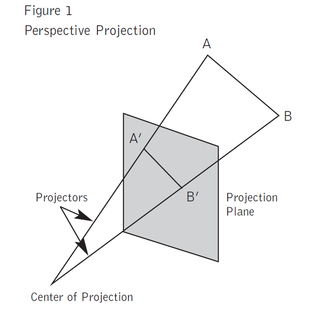
The idea of trying to present the illusion of a 3D picture on a 2D surface had its beginnings in the Renaissance. The painters of the period utilized the idea of a “point at infinity” to represent the place where parallel lines seem to intersect. Mathematicians, in their attempts, to prove Euclid’s parallel postulate developed non-Euclidean geometries5,6 – geometries that do not assume one or more of Euclidean Geometry’s postulates – provided firm mathematical foundations for this idea of a “point at infinity.” When we attempt to represent a 3D object on a graphics device, we are utilizing these concepts. There are two types of projections that are commonly used to create these representations: perspective and parallel. If the distance from the center of the projection to the projection (or view) plane is finite, then the projection is perspective; if the distance is infinite, the projection is parallel. Perspective projections do not preserve angles and distances, while parallel projections do. Figure 17 provides an illustration of the two basic projection types. Since it is the perspective projection that creates the more “realistic” representation, the illusion of 3D, it is this projection method that we will discuss here.

We start by assuming that the projection plane is perpendicular to the z axis and is located at z = d.The center of projection is at the origin. To determine the projection Pp = (xp , yp, zp)T of a point P = (x, y, z)T we use similar triangles to get xp = xyz/d,
yp = yyz/d, and zp = d.The division by z causes the projection of more distant objects to be smaller than that of closer objects.

A more general formulation was developed by N. Weingarten.7 We summarize this formulation here. We still assume that the projection plane is perpendicular to the z axis and is located at z = zp, but now the center of projection is a distance Q from the point (0,0,zp)T, the intersection of the projection plane with the z axis. If the normalized direction vector from (0,0,zp)T to the center of projection is (dx, dy, dz)T then it can be shown that the projection Pp can be computed by a simple matrix product. This formulization is given in Exhibit 5 on the Conference Abstracts and Applications CD-ROM. This matrix transformation provides a one-point perspective projection. The vanishing point (or the point at infinity) is given by (Qdx, Qdy, zp)T.

There are many variations of this type of projection; for example, those that allow for multiple vanishing points. A summary of the mathematical effort required to transform a 3D world coordinate into a 2D device coordinate is given in Figure 27.

Section 3: A Little Light on the Subject

When considering the lighting of a scene, one must consider the interaction of light with the surface of an object in the scene and model this interaction. One must consider the light emitting sources (a point source or distributed source) as well as the light reflecting sources (ambient light or background light). There are also two types of reflection to be considered: diffuse and specular. In diffuse reflections, incoming light that is not absorbed is reflected off the surface in random directions, while in specular reflections the light reflects in a nearly fixed direction without any absorption.

In order to compute the overall illumination of a given point P = (x, y, z)T, we need the following information:

1. The direction of the light source L (there could be more than one)
2. The normal vector N
3. The reflection vector R (there could be more than one)
4. The viewing vector V

If S = (Sx,Sy,Sz)T is the position of the light source and E = (Ex,Ey,Ez)T is the position of the eye, then L = S – P and V = E – P. Each of L and V must be normalized, i.e., made to have length one. The computation of N and R can be complicated depending on the type of surface. N and R must also be normalized. Once L, V, N, and R have been determined then cosw = L•N and cosu = V•R and the Phong8 model of illumination can be computed by9:

I* = Ia*kd*+ Ip*(kd*cosw/d + kscosnu)

where
* = r, g, or b (for red, green, or blue)
Ia* = intensity of ambient light for *
kd* = diffuse reflectivity of *
ks = a constant that estimates the specular reflection coefficient (0 # ks # 1)
Ip* = intensity of point source of light for *
n = measure of “shininess” of the surface, very shiny = large n ( > 150)
d = distance to the point source or distributed source of light

There are many other models that could be considered, for example, GOUR7110, WARN8311, VERB8412, and NISH8513.

Section 4: The Spline’s the Thing

When trying to represent an object mathematically, quite often it is impossible to construct an appropriate model using only simple geometric shapes. If this is the case, then arbitrary curves need to be created to model the object. The curves of choice are splines and other parametric curves. These curves are used in animation to generate in-between frames, or to create curves when only a few datapoints describing the curve are known. Yet another application of these curves is the generation of arbitrary surfaces. Each of these applications has essentially the same premise: from a few data points, generate a smooth curve based on this data. This curve should be simple to compute and easy to modify if a change in data is necessary.

Parametric equations are used to represent curves that are not easily represented or are impossible to represent by a function. Examples of this would be curves that have loops or places of infinite slopes. In this case we use a parameter, say t, and describe each variable x and y as functions of t, x = x(t) and y = y(t), over some range of t. If we are working in three dimensions then each of x, y, and z would be parameterized. The slopes of tangential lines for parametric curves are simple to compute. For example, dy/dx = (dy/dt)(dt/dx) = (dy/dt)y(dx/dt), i.e. the chain rule of differentiation becomes simply a quotient.

Splines are piece-wise defined polynomial functions of, usually, low degree. If you have data points (x0, y0), … (xn, yn), xi s distinct, then the Natural Cubic Spline, S(x), will interpolate this data (i.e., S(xi) = yi ) and is given by cubic polynomials defined on each of the intervals [xi, xi+1], i = 0,…, n-1.To determine the coefficients of this spline, one must solve an (n-1)x(n-1) tridiagonal linear system of equations. This spline, though historically significant, is not very useful in computer graphics. A unique spline does not exist if there is a repeated x value and if a data point needs to be changed then the entire spline will need to be recomputed.

To overcome these problems, splines that do not necessarily interpolate the given data are used. The most often used splines are the Bézier14,15 and uniform B-splines.16 Splines can be defined for any degree, though the cubic splines are usually sufficiently robust to handle the smoothness requirements in graphics.

The uniform cubic B-spline, b, stretches over five data points, called knots. The distances between the knots are all taken as 1 and the point 0 is put in the middle of these five knots to achieve symmetry. Formally this is given by:

b(u) = 0 if u ≤ -2
b(u) = (2 + u)3 / 6 if -2 ≤ u ≤ -1
b(u) = (2 + u)3 / 6 – (2 + u)3 / 3 if -1 ≤ u ≤ 0
b(u) = 2(1 – u)3 / 3 – (2 – u)3 / 6 if 0 ≤ u ≤ 1
b(u) = (2 – u)3 / 6 if 1 ≤ u ≤2
b(u) = 0 if 2 ≤ u

If we need to draw a curve based on knots P0 = (x0, y0, z0), … Pn = (xn, yn ,zn), then one way to construct the approximating curve is to form the linear combination: where pi stands for xi, yi , or zi. The most convenient way to draw the B-spline curve is
to use a matrix product. This product expresses the value of C in any subinterval [ui,ui+1] with i not 0 nor n-1 and is given as Exhibit 6 on the Conference Abstracts and Applications CD-ROM.

As the parameter u changes from 0 to 1 the formula generates the curve from Pi to Pi+1. The other most commonly used cubic spline is the Bézier spline. The main difference between the two is that the Bézier curve is globally, not locally, controlled by the
points Pi. Changing one of the control points affects the entire Bézier curve, but its strongest affect is in the neighborhood of the point. The matrix formulation of the Bézier curve is given on the Conference Abstracts and Applications CD-ROM as Exhibit 7.

To generate spline surfaces, one simply takes the Cartesian product of two splines. For example, we define a B-spline surface b(u,v) = b(u)b(v).The matrix formulation of this surface is given by S(u,v) = 1/36UMPMTVT where U = (u3,u2,u,1), V =(v3,v2,v,1) and

A similar formulation for Bézier surfaces exists.

There are, of course, other splines and generalizations that can be used to model curves or surfaces, e.g., Hermite, non-uniform B-splines, and Beta splines.

Section 5: Other Neat Stuff

We have only begun to scratch the surface of the different types of mathematics used in computer graphics, and we have omitted many of the details of the concepts presented in this paper. For example, most of the calculus concepts involved in the illumination section were omitted. However, it should be fairly obvious that geometry, linear algebra, and calculus play fundamental roles in the representation and manipulation of images. Other aspects of computer graphics often utilize more complicated mathematics. For example, antialiasing uses digital signal processing and hence Fourier transforms, and physically based modeling requires the solution of partial differential equations. To truly understand fractals, complex arithmetic and a little analysis will go a long way. In order to fully appreciate and understand the finer aspects of computer graphics one must at least appreciate, if not understand, the finer aspects of mathematics, as you would not have one without the other.

Many types of math (geometry, algebra, and calculus, among others) are crucial “tools of the trade” for people who create computer-generated effects. For example, animating people and creatures calls on methods from geometry and trigonometry. Rendering actual images requires algebra and arithmetic, among other things. And simulating physical phenomena like cloth and water uses knowledge from calculus. This presentation shows some examples from film and commercial effects that illustrate the use of these mathematical tools.