“1991 Education Slide Set”, 1991
Title:
- 1991 Education Slide Set
Year:
- 1991
Conference:
Description:
SIGGRAPH ’91 Educators’ Slide Set Credits
Edited by Steve Cunningham
SIGGRAPH ’91 Educators’ Program Chair
Diana Tuggle
SIGGRAPH Visual Image Editor
The educators’ slide set provides instructors with slides that support common subjects in computer graphics courses at all levels. The set, covering three topic areas, has 78 slides. Representative slides are printed here in black and white. The full color 35mm slide set can be order from: ACM order department, P.O. Box 64145, Baltimore, MD 21264; 1-800-342-6626. The ACM order number for the SIGGRAPH ’91 educators’ slide set is 915913. The cost is $33 for members; $44 for non-members.
Ray tracing
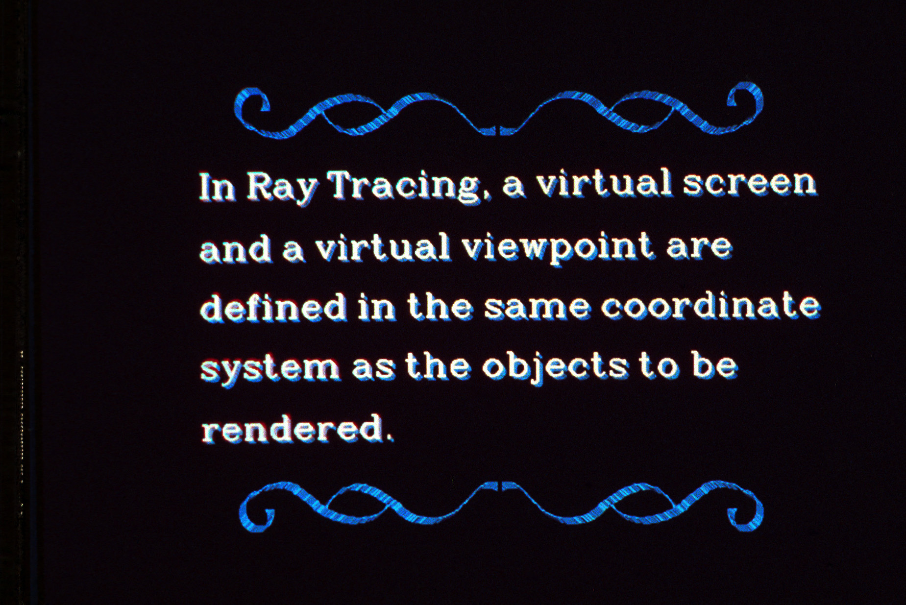
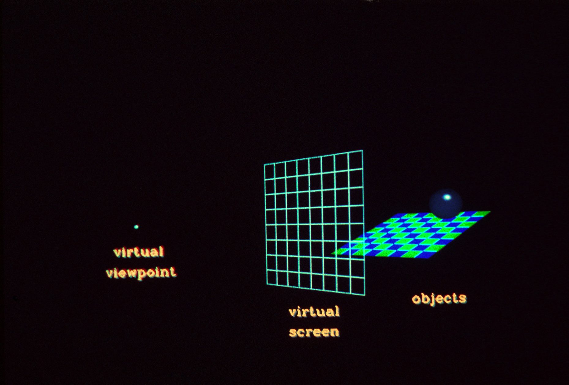
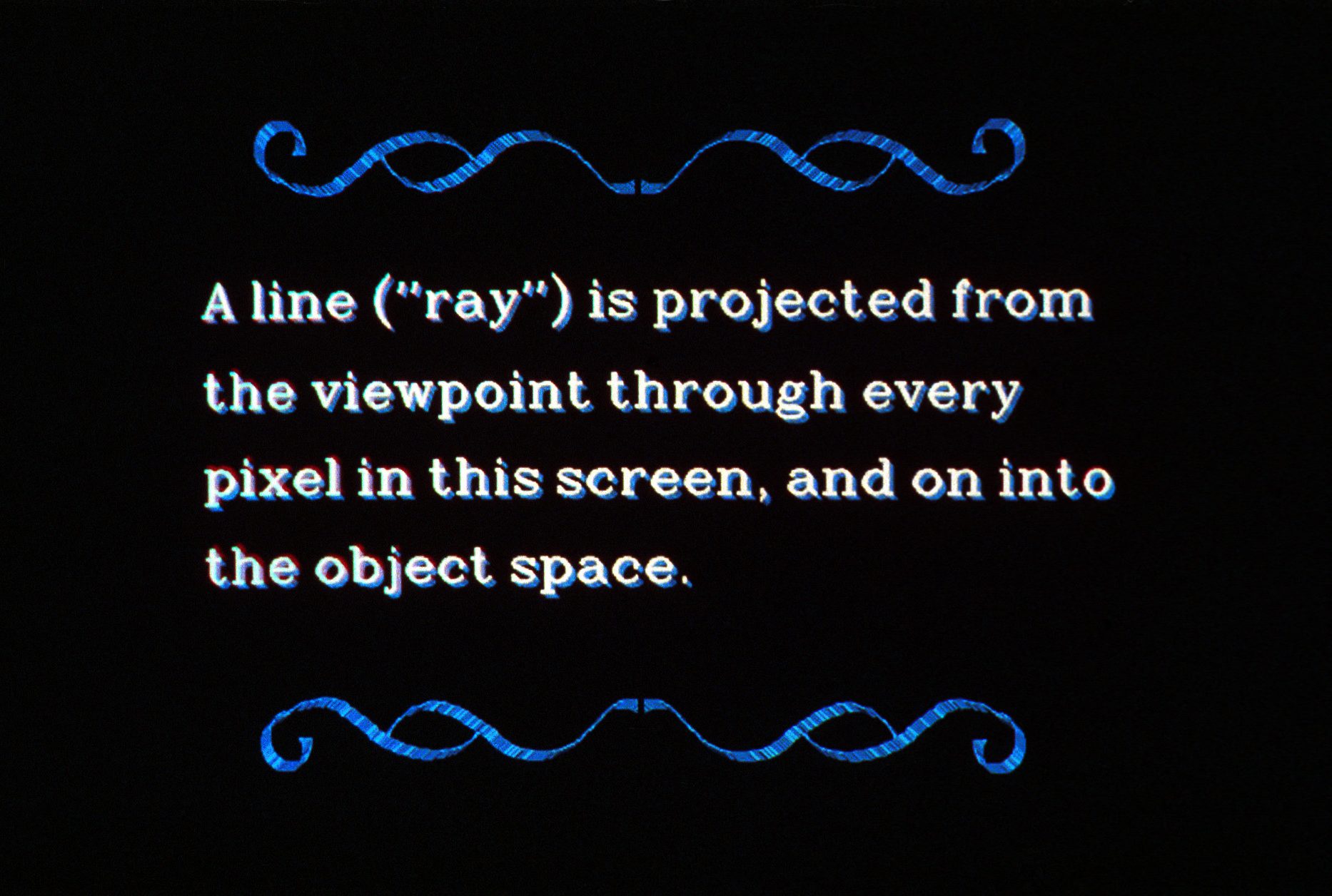
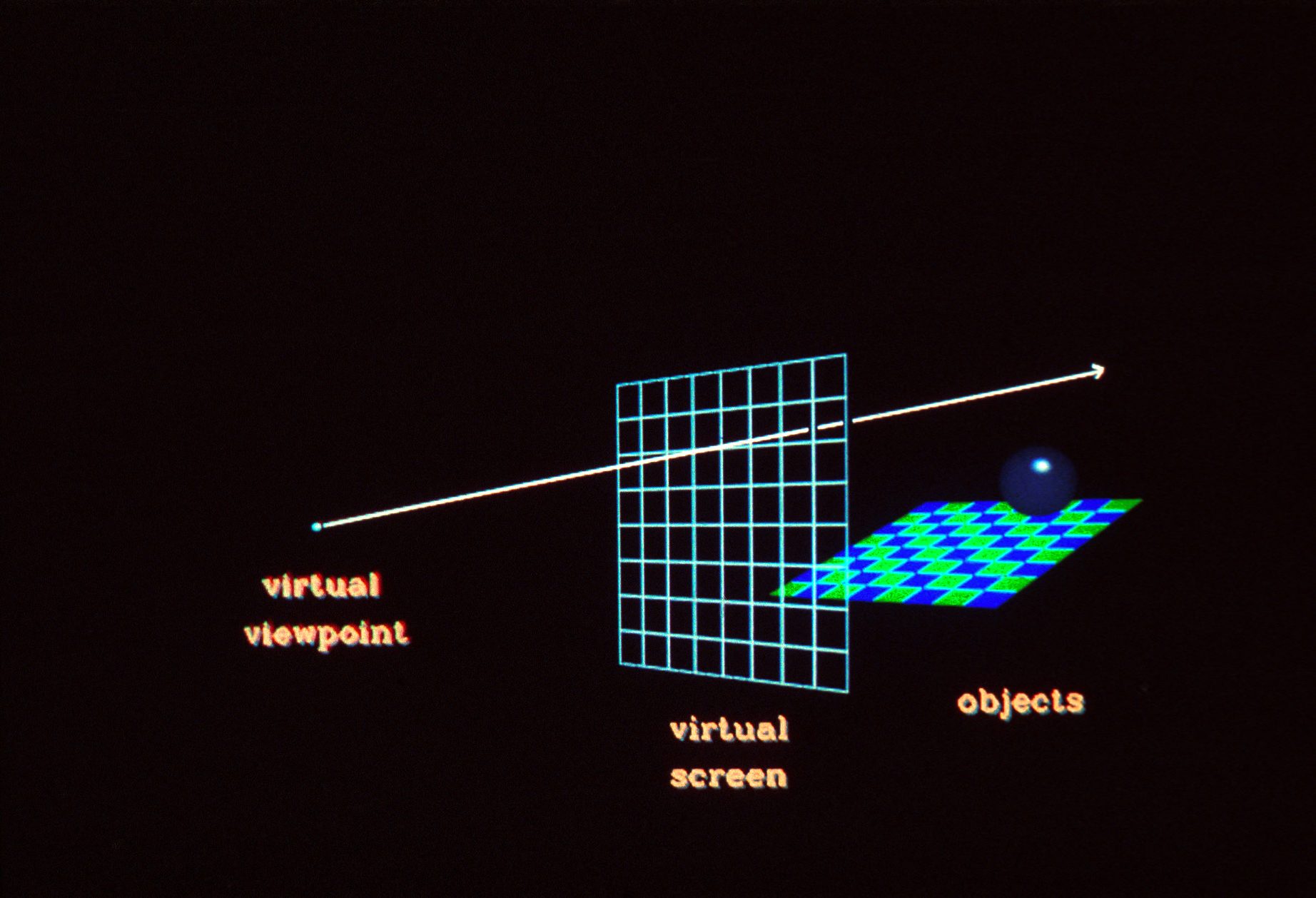
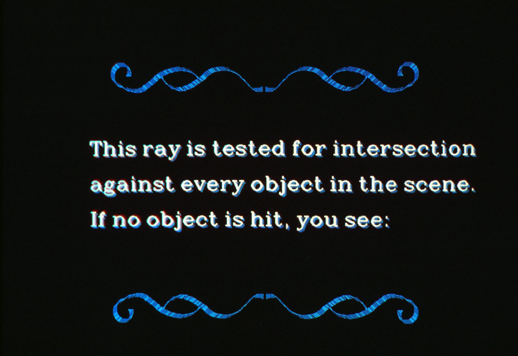
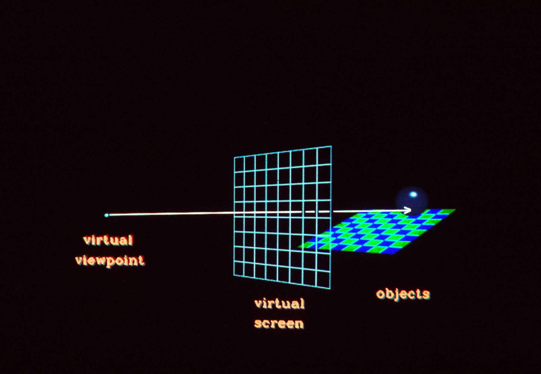
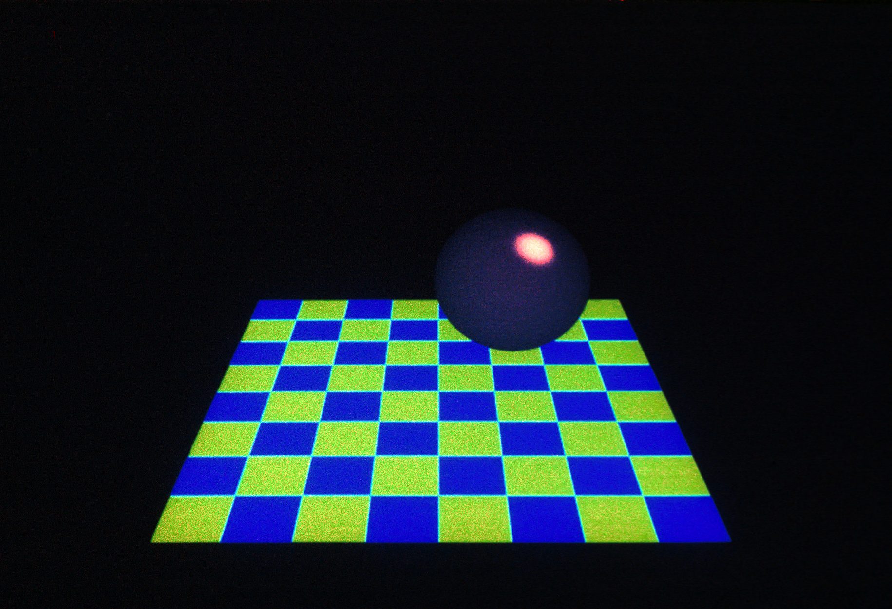
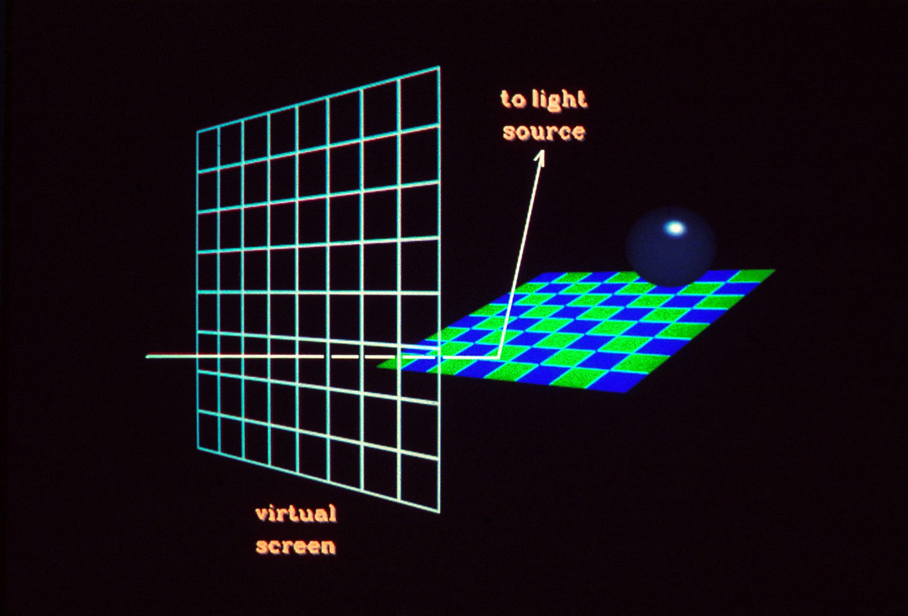
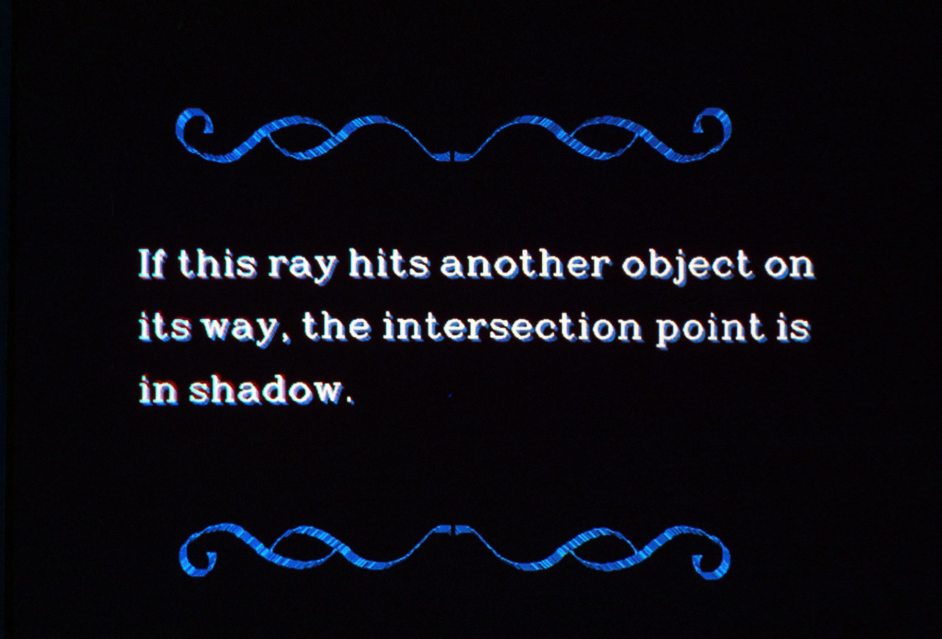
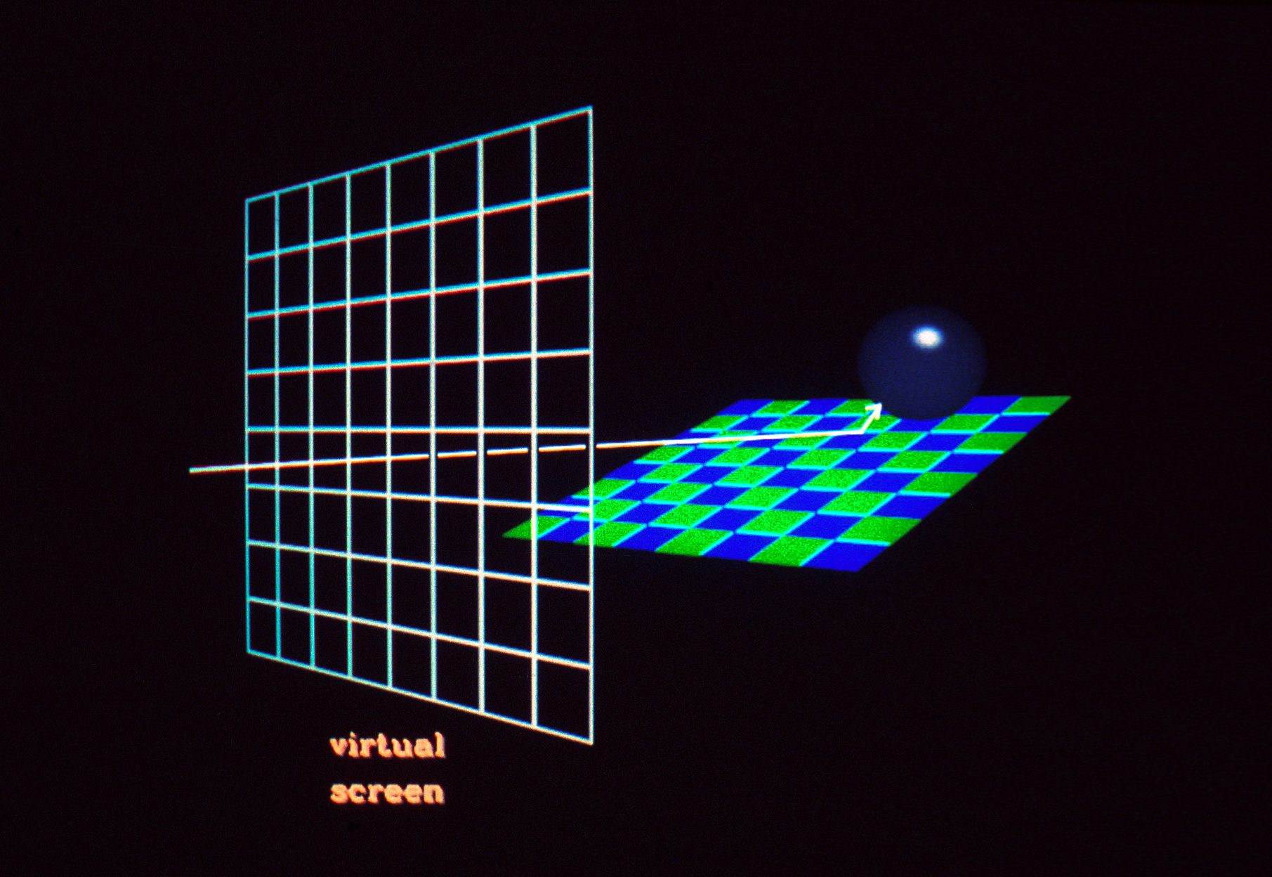
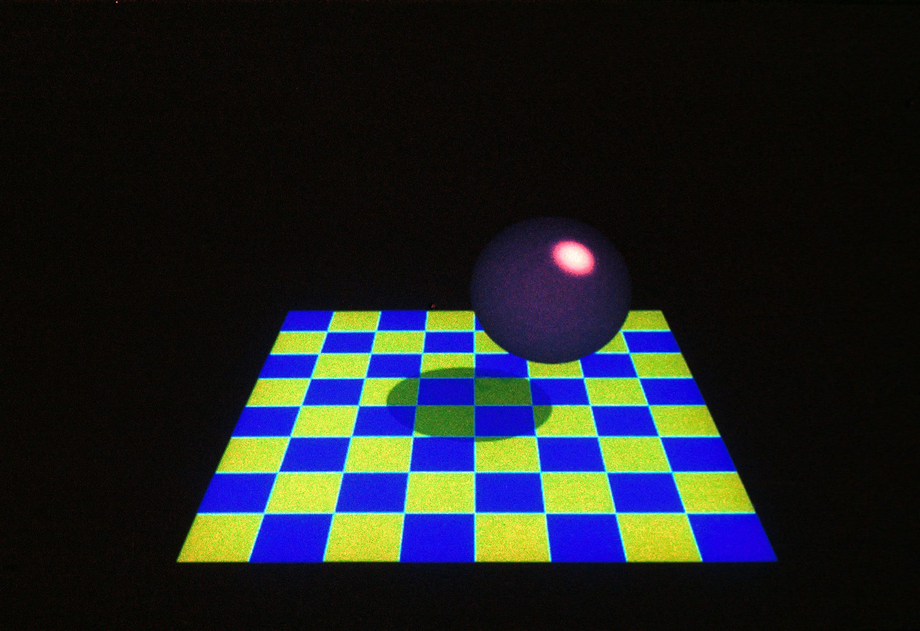
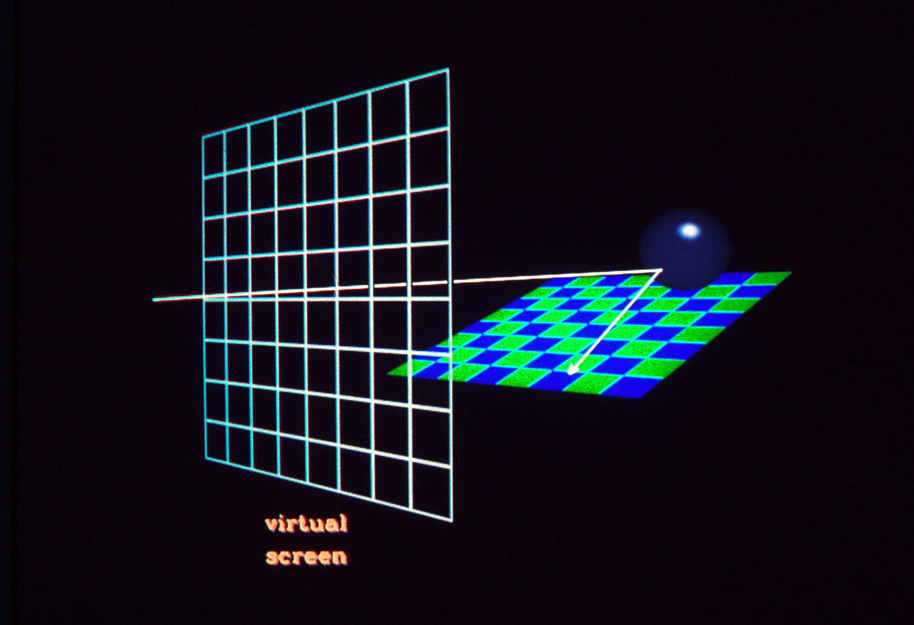
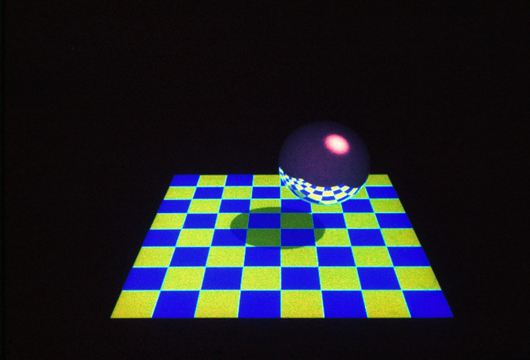
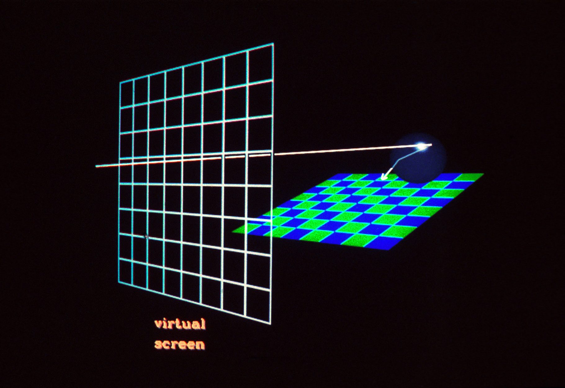
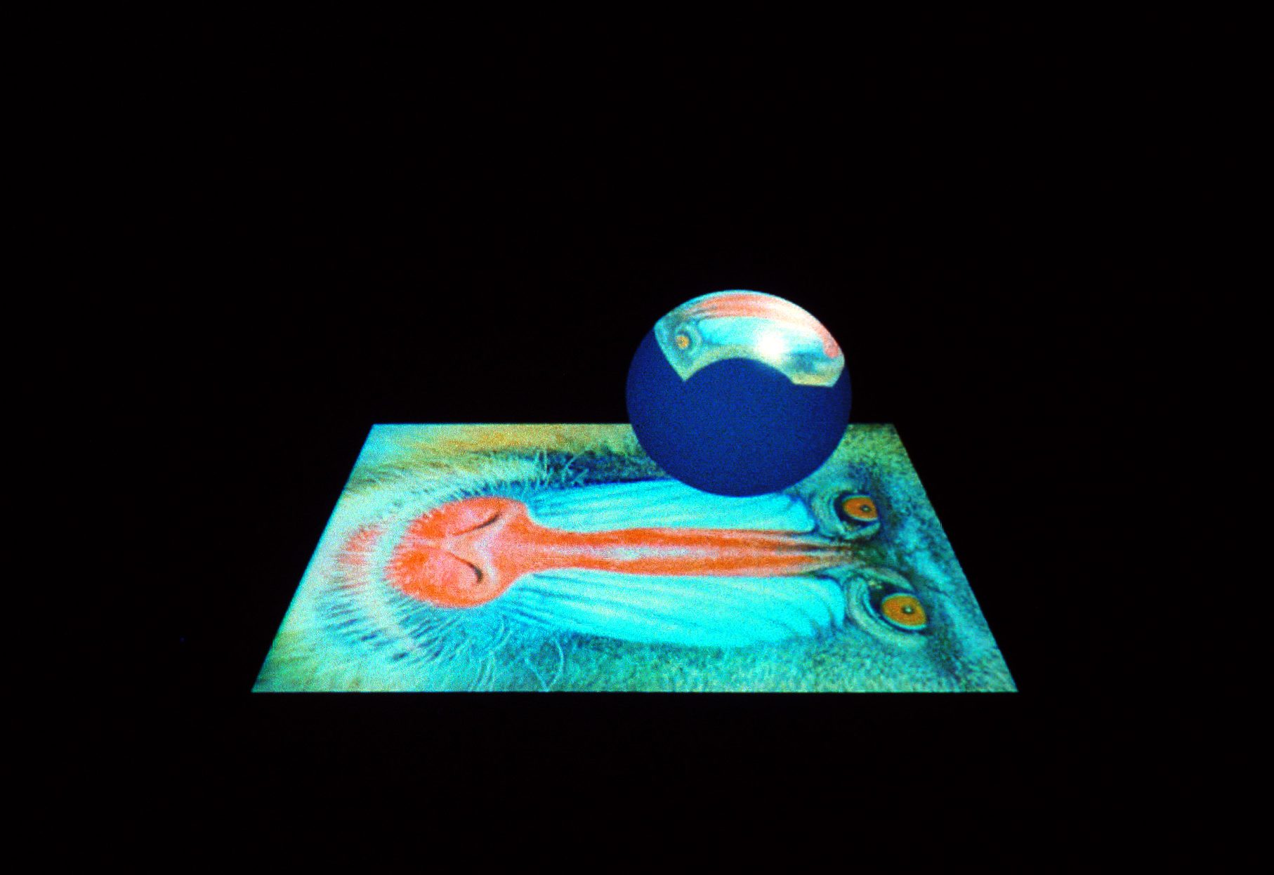
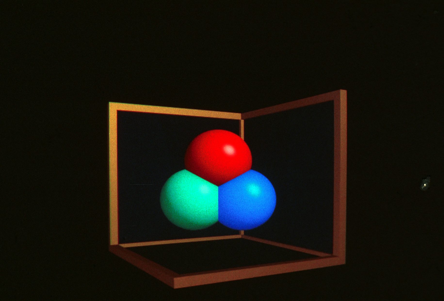
Slides 1 through 27. Produced by Michael Sweeney with the help of David Forsey, David Martindale and Robert Krieger, University of Waterloo. Copyright 1984, University of Waterloo. These are slides from the video, “Ray Tracing: A Silent Movie and Some Slides,” SIGGRAPH Video Review #14, 1985. They give a good introduction to the fundamental principles of ray tracing, and also have historical value. We suggest that interested instructors also get a copy of the Video Review for class use.
Projections
Slides 28 through 54. Produced by Norma Fuller and Przemyslaw Prusinkiewicz of the University of Regina. Copyright 1991, Fuller and Prusinkiewicz. This series contains 26 slides illustrating various aspects of projections for computer graphics. After the introduction slide (#28), the slides illustrate the following principles.
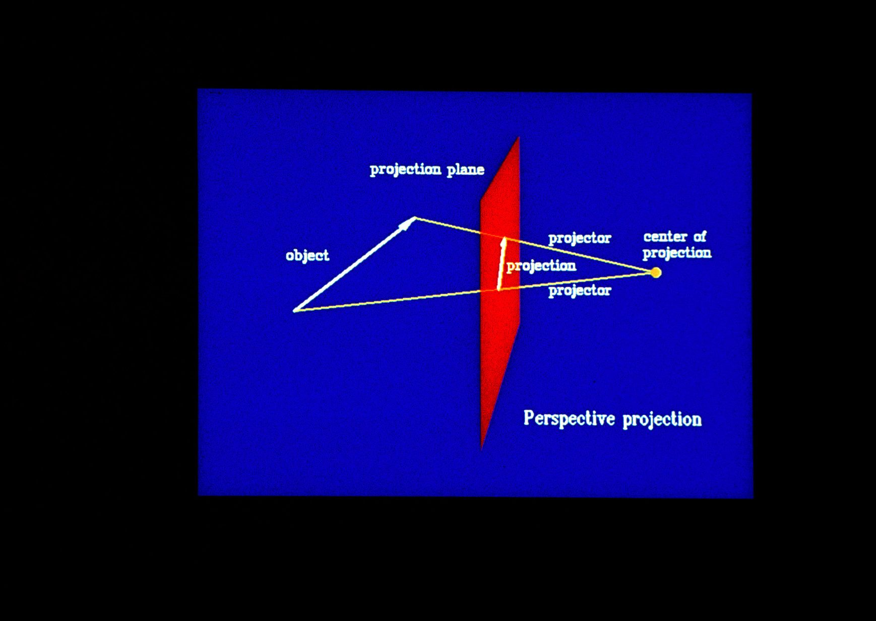
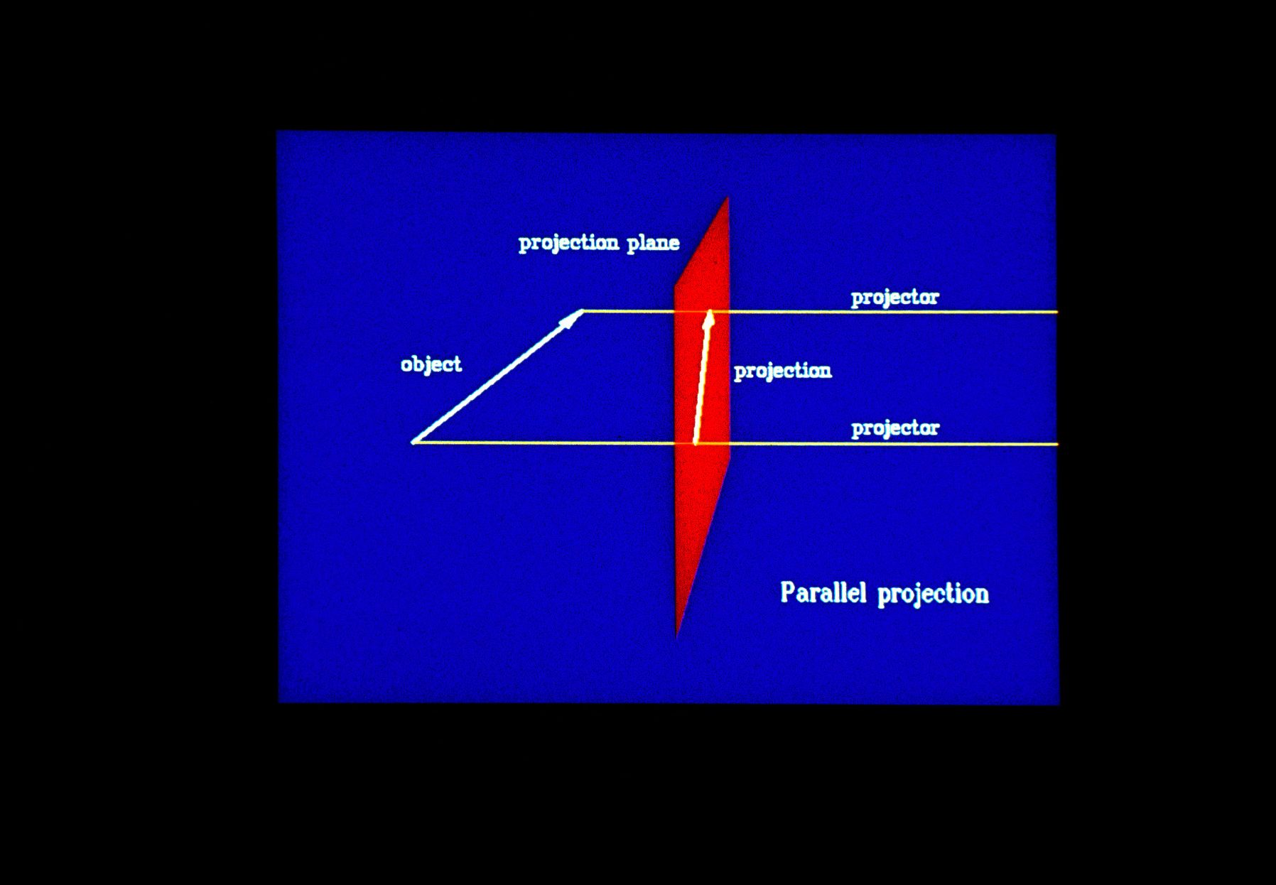
29. In order to draw a three-dimensional object on a two- dimensional surface, a projection must be performed. A projection is defined by straight line projector rays emanating from a centre of projection, passing through each point of the object and intersecting a projection plane to form the projection.
30. There are two kinds of projections-parallel and perspective. The distinction lies in the distance between the centre of projection and the projection plane. If the distance between them is finite, the projection is perspective while if the distance between them is infinite, the projection is parallel.
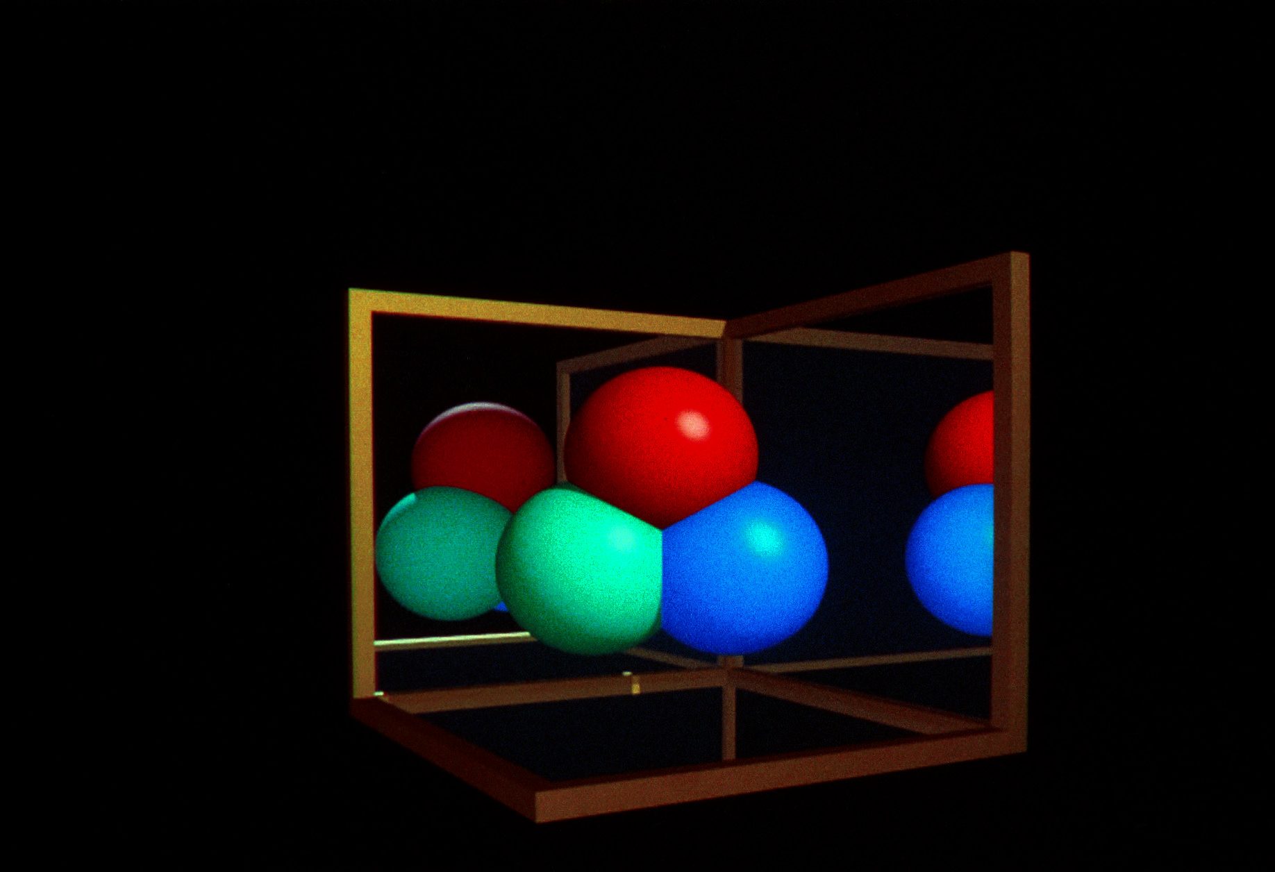
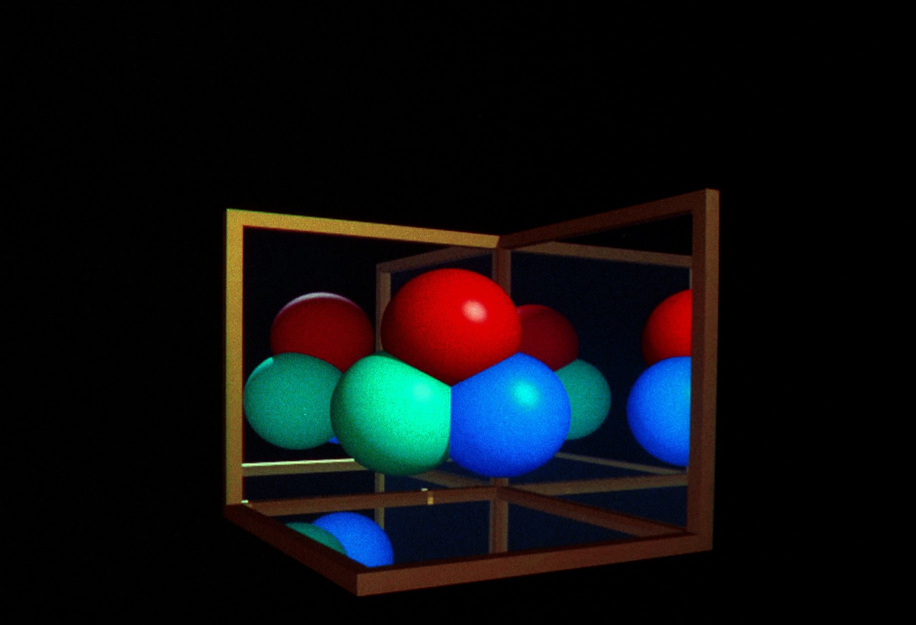
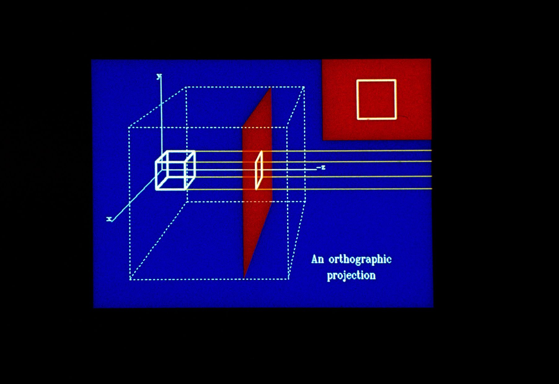
31. There are two types of parallel projections based upon the relation between the projector rays and the normal to the projection plane. In orthographic parallel projections, they are parallel.
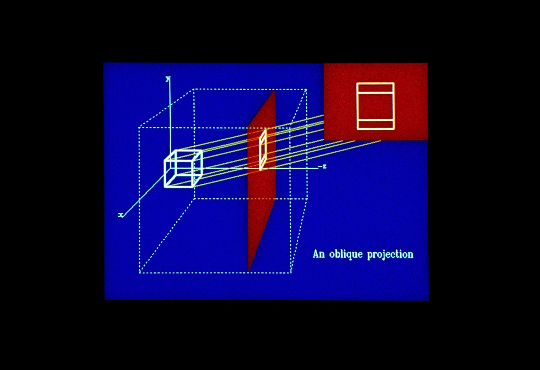
32. In oblique projections, they are not.
33. Notice that the parallel edges of the object remain parallel in the projection. Angles are preserved on the faces of the object that are parallel to the projection plane.
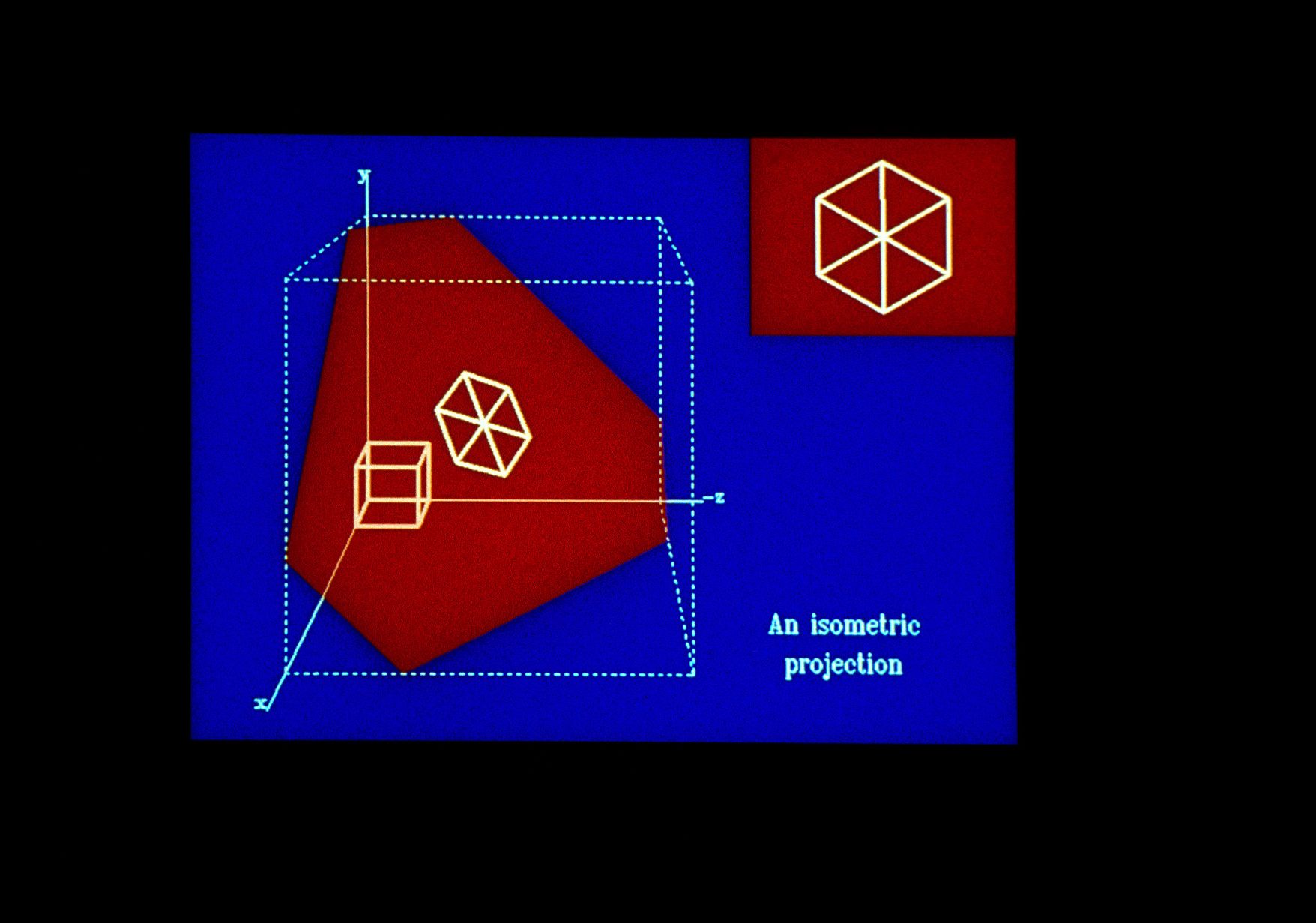
34. A special case of orthographies projection is one in which the projection plane normal makes equal angles with all the principal axes. It is called an isometric projection. All three principal axes are equally foreshortened allowing measurements along the axes to be made with the same scale.
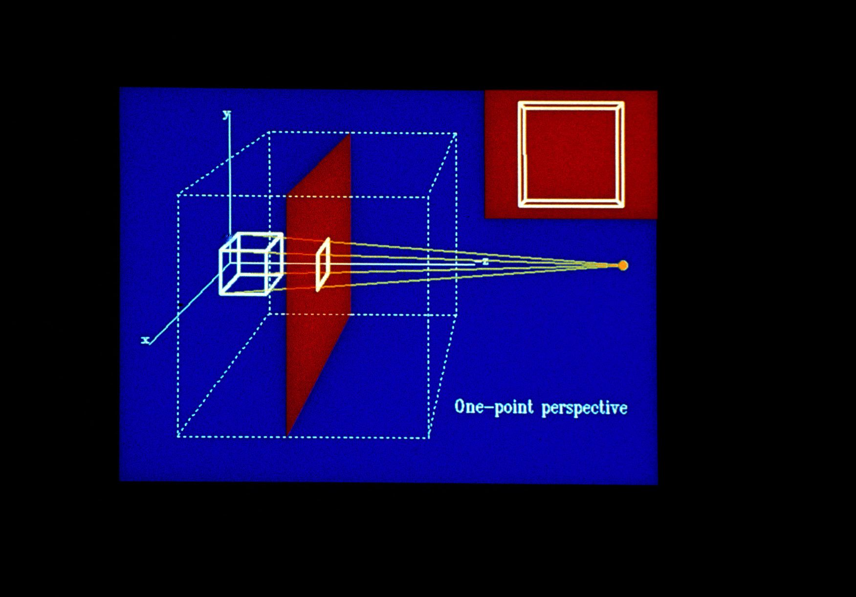
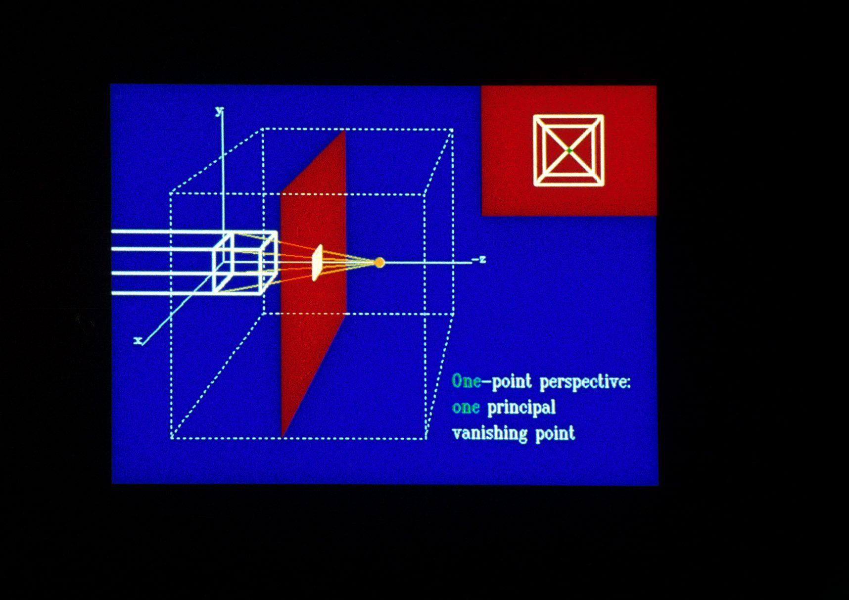
35. Perspective projection creates an effect similar to the human visual system. Perspective projections are categorized according to the nuinber of principal axes that the projection plane cuts. One-point perspective cuts one principal axis.
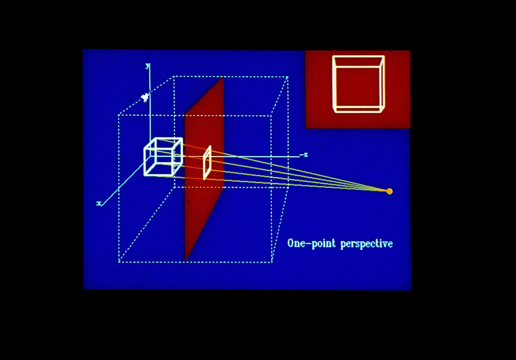
36. In this slide you can see the effect of moving the centre of projection down with respect to the position depicted in the previous slide.
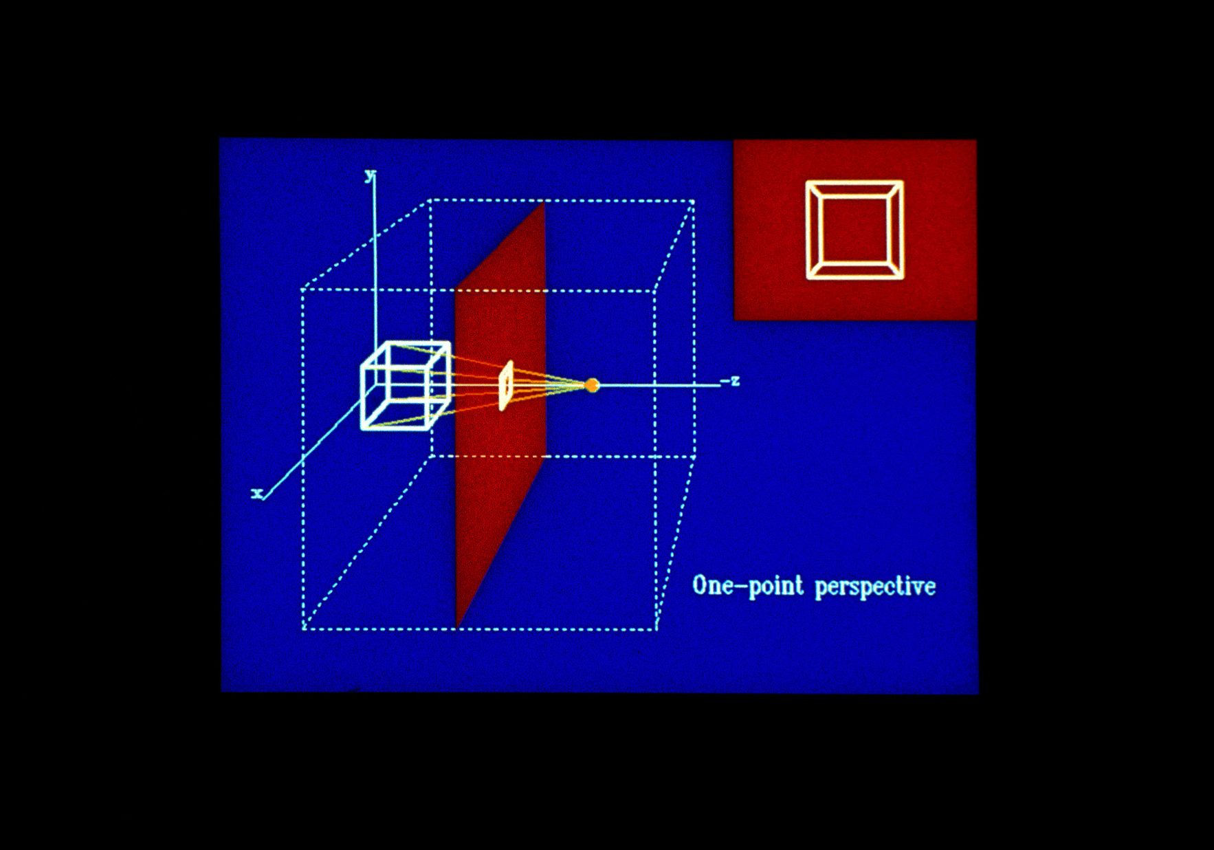
37. In this case the centre of projection is moved closer to the projection plane.
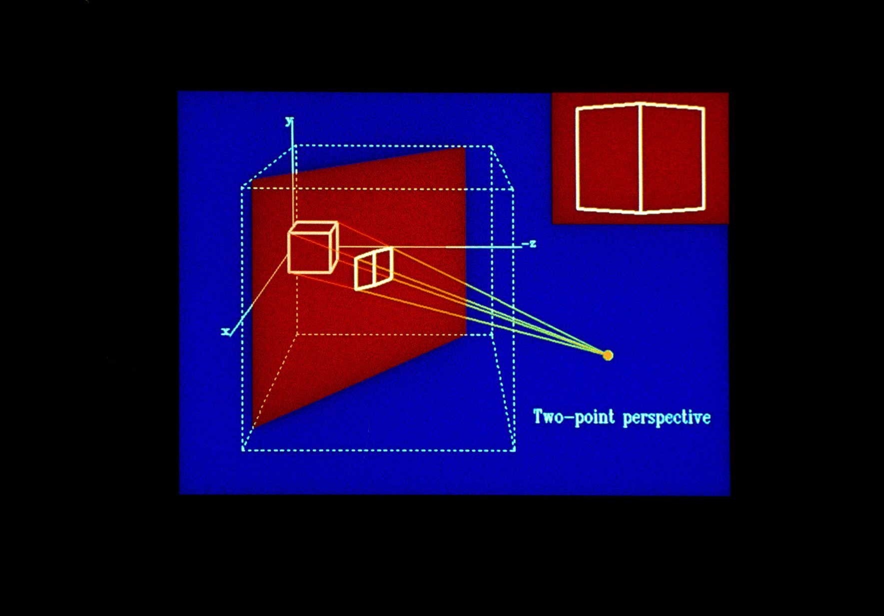
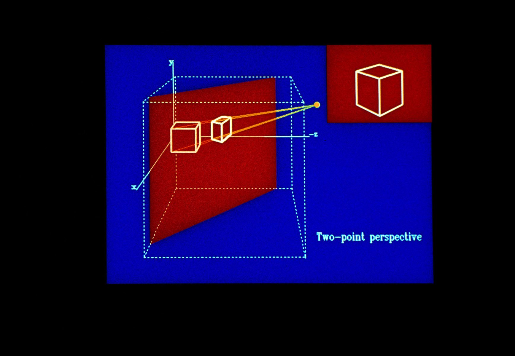
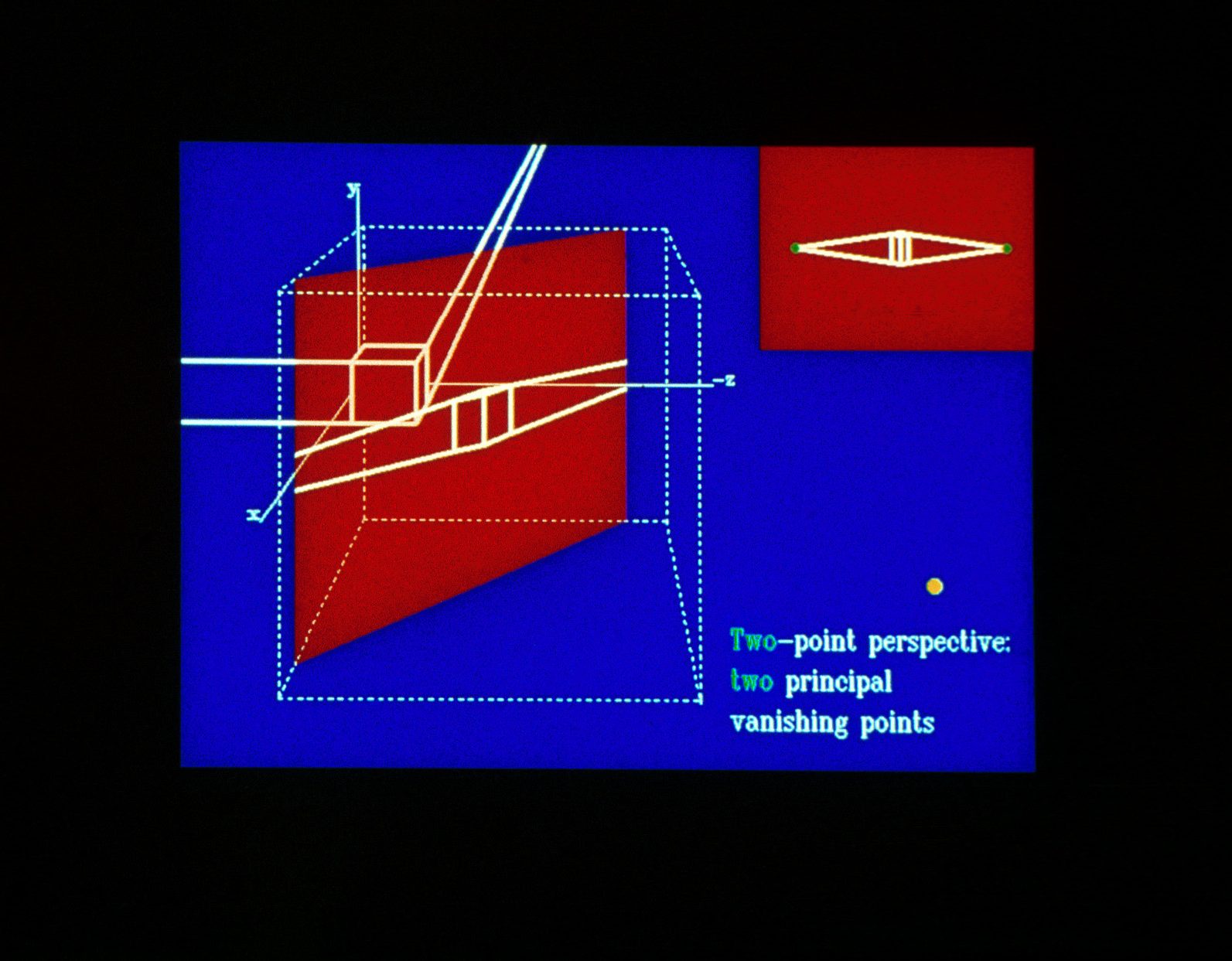
38. In this slide we have two-point perspective – the x and z axes are cut by the projection plane.
39. Another view of two-point perspective.
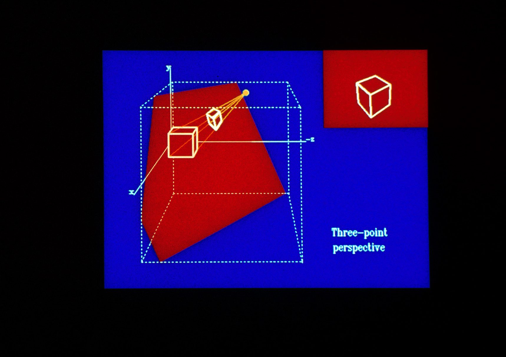
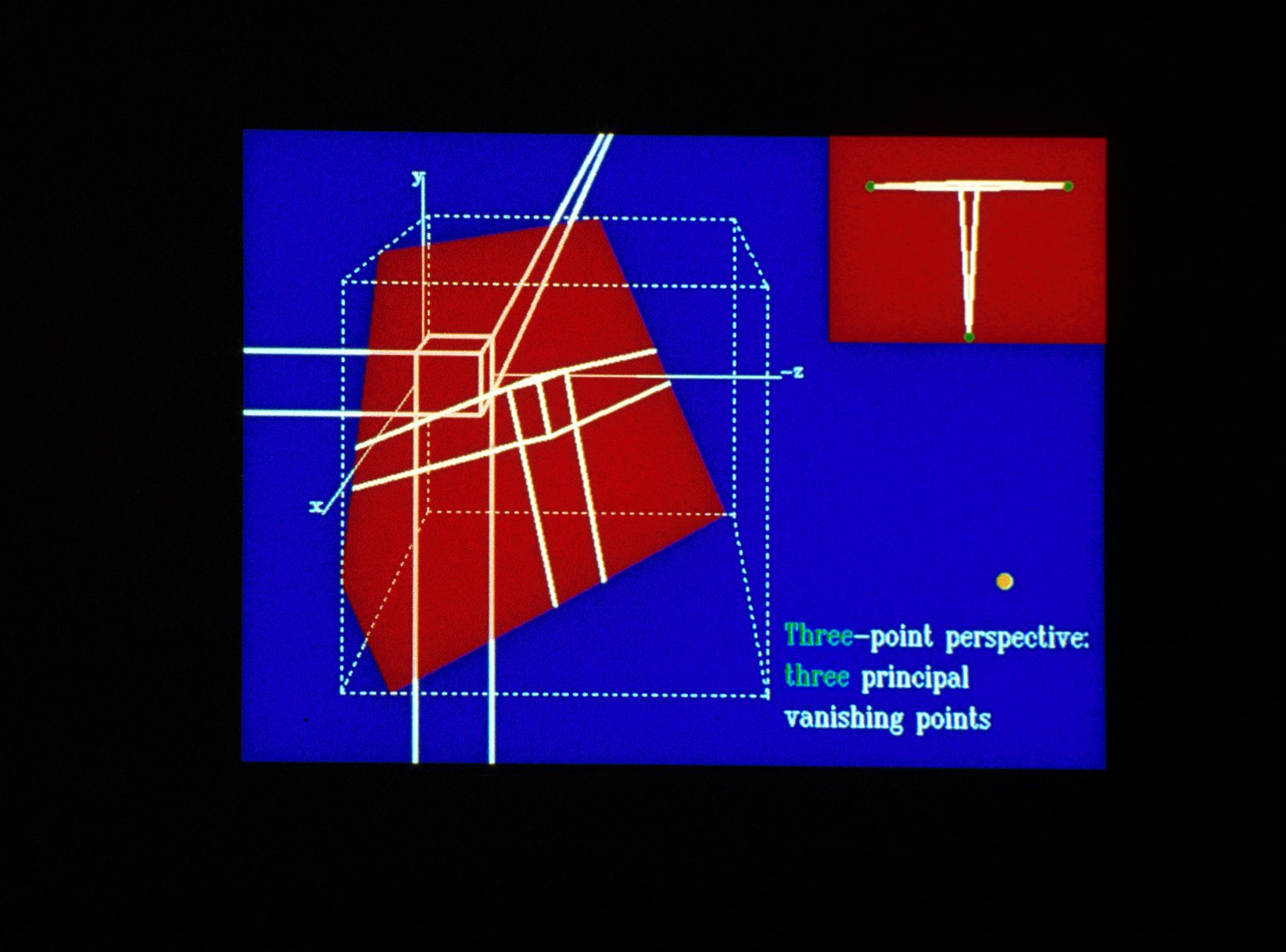
40. In this case all three axes are cut by the projection plane. So we have three-point perspective. In perspective projections any set of parallel lines which are not parallel to the projection plane will converge to a vanishing point. If the set of lines is parallel to one of the principal axes, the point is called a principal vanishing point. There are at most three principal vanishing points.
41. In one-point perspective there is only one principal vanishing point.
42. In two-point perspective there are two principal vanishing points.
43. In three-point perspective there are three principal vanishing points.
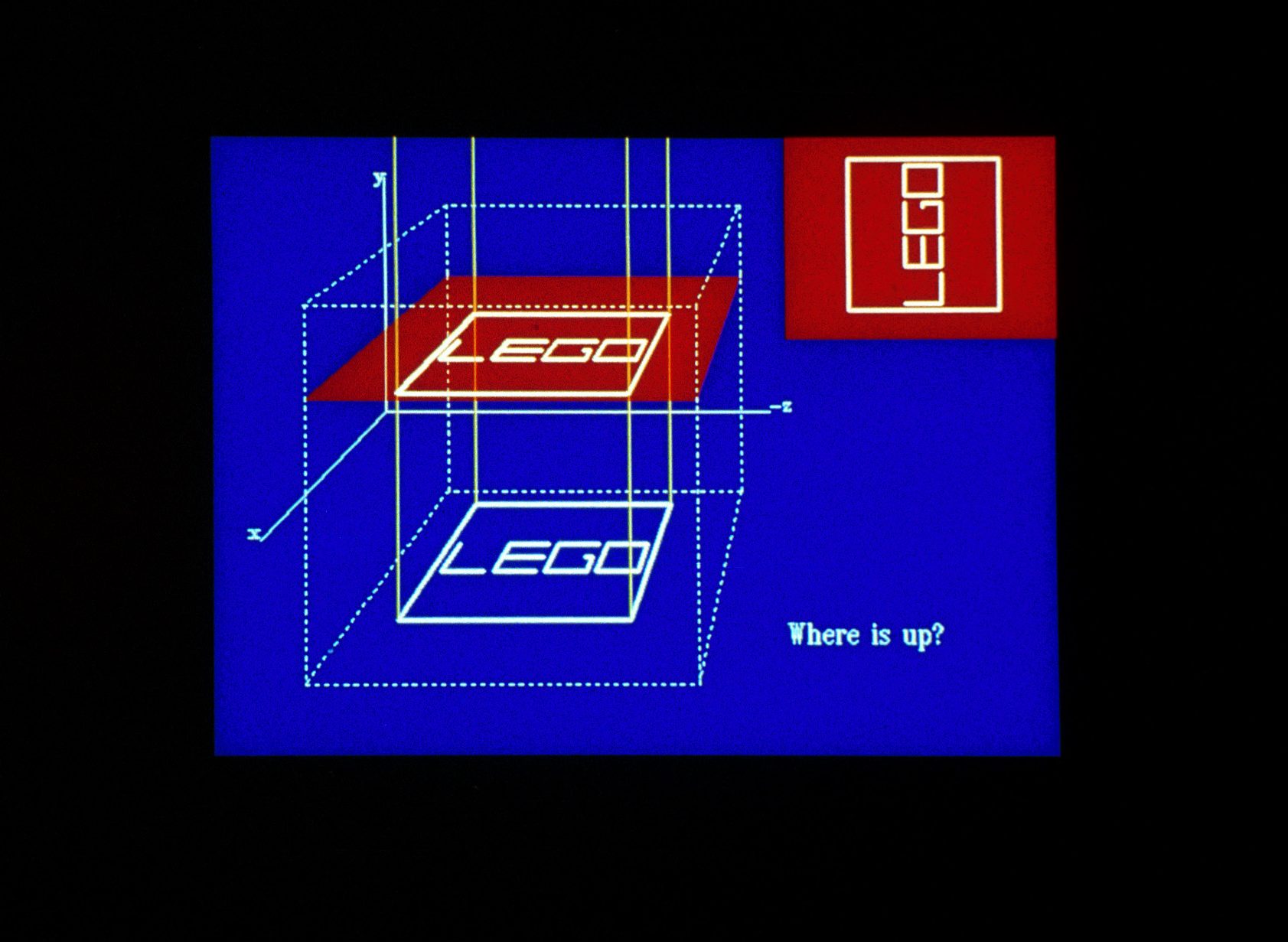
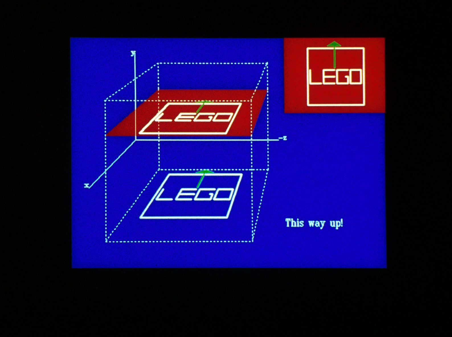
44. Here is a viewing example in which the results were not as expected (the image appears on the screen placed vertically rather than horizontally). So we see that there is more to viewing in three dimensions than just intersecting the projector rays and the projection plane. For example, it is necessary to indicate which direction will appear as “up” on the screen. The following slides show how this can be accomplished.
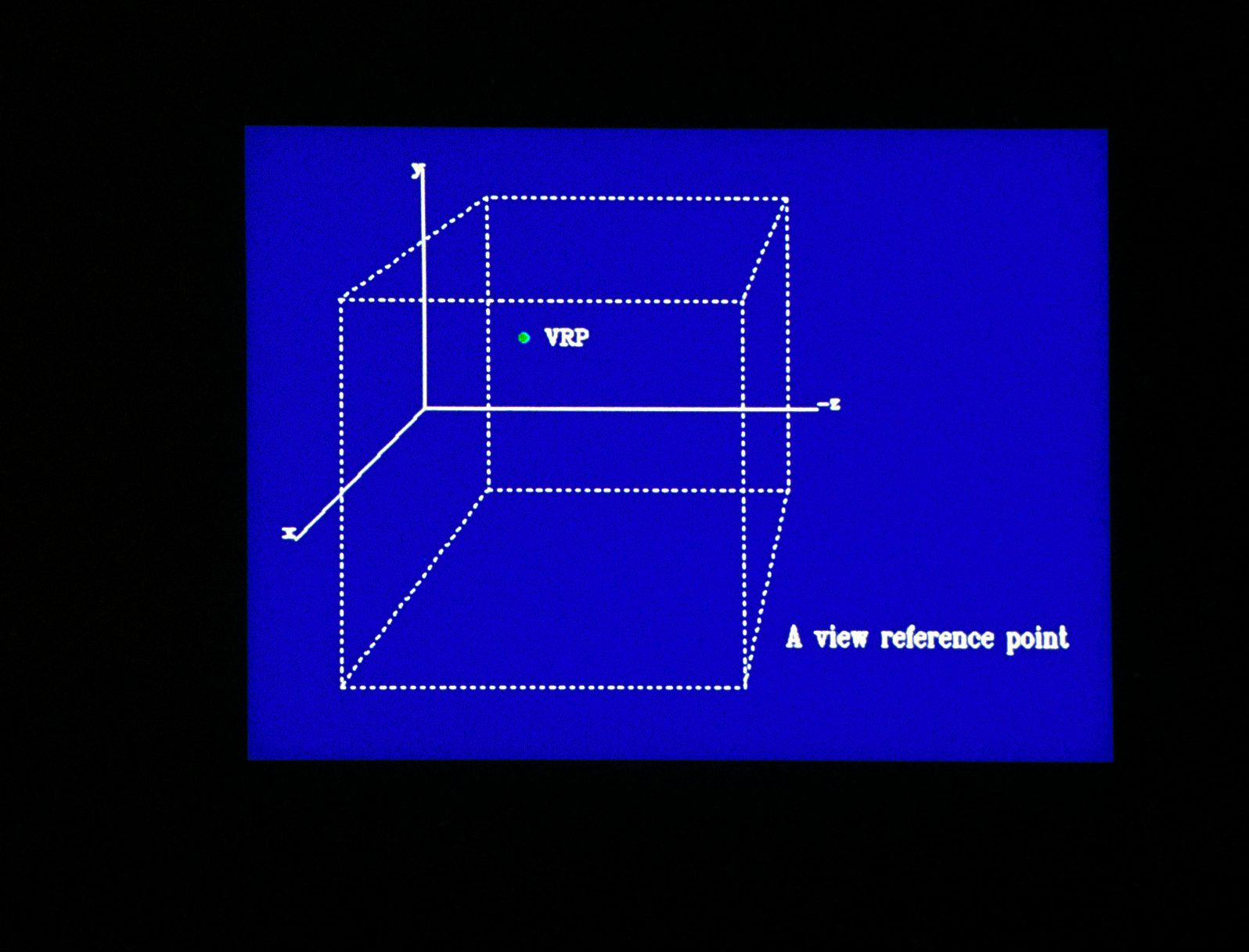
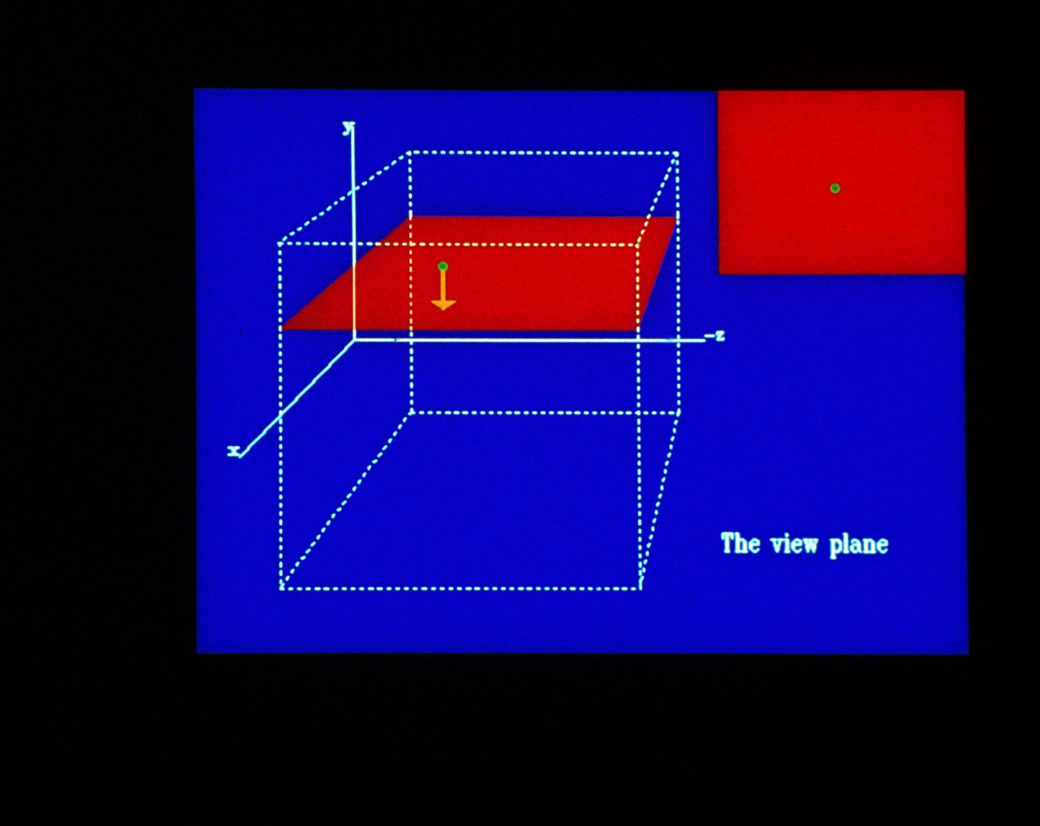
45. The first problem is to define the position of the projection plane (also called the view plane) in space. We accomplish this by first defining the view reference point (VRP) which will lie on the plane.
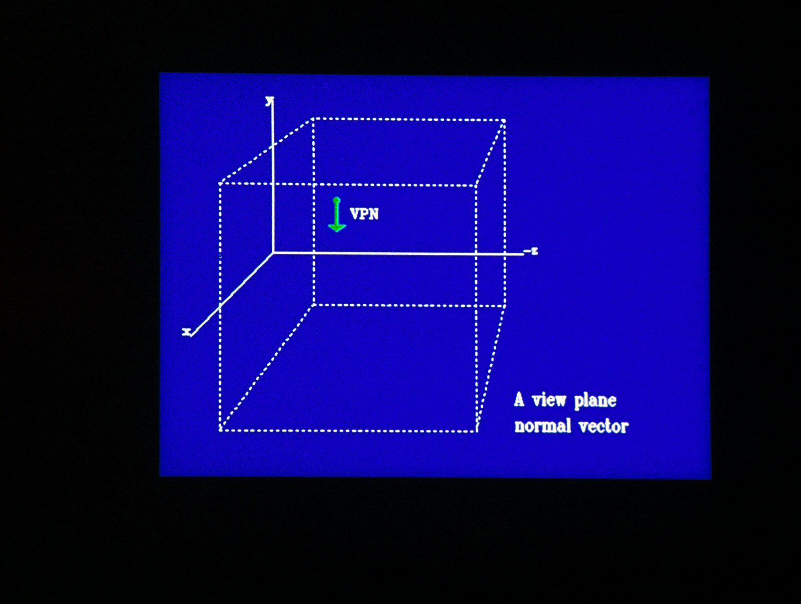
46. Then we define a view plane normal vector (VPN).
47. They are sufficient to define the view plane.
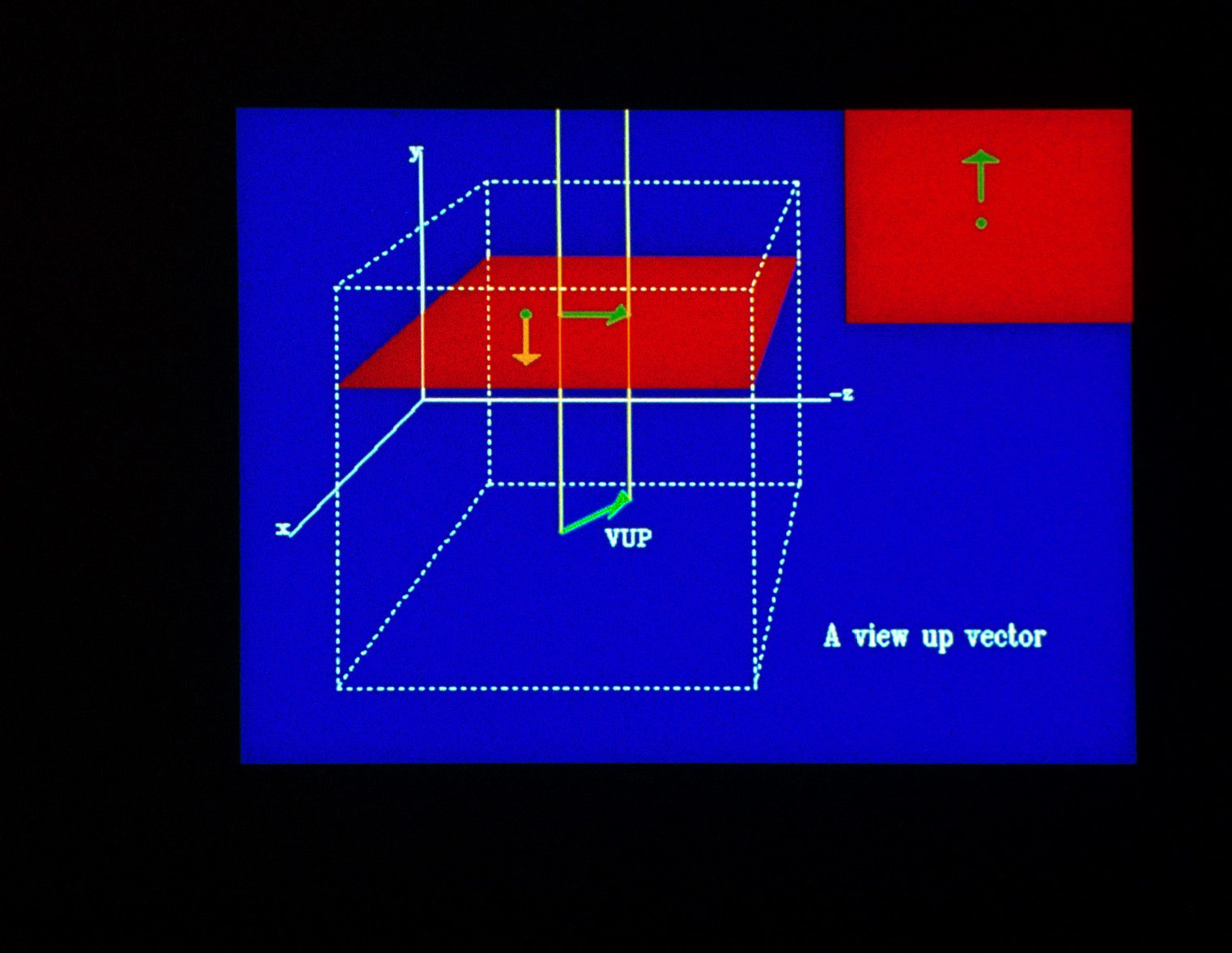
48. We also need some way to say which direction is “up” on the view plane. We define a three-dimensional vector called the view up vector (VUP) and take a projection of it onto the projection plane. This determines the direction “up” on the view plane.
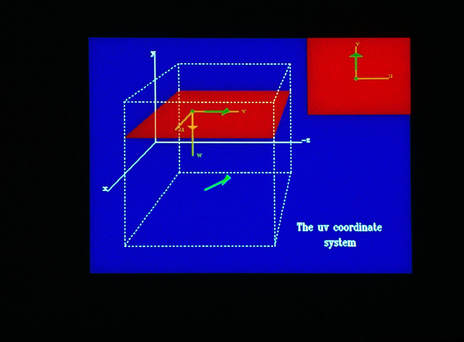
49. Using the projection of the view up vector, the view reference point at the coordinate centre and the view plane normal, we can set up a left-handed coordinate system on the view plane called the uvw-system.
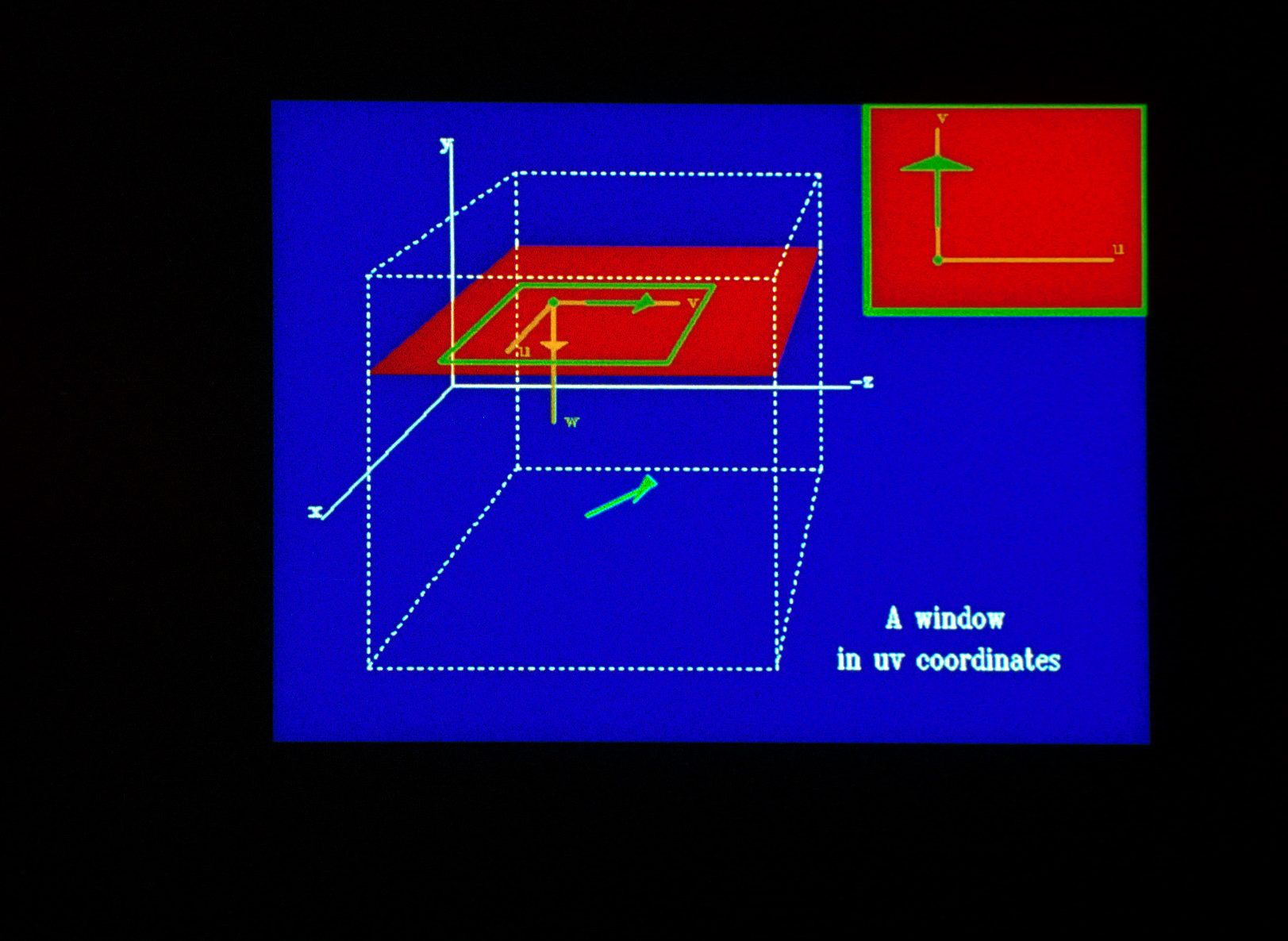
50. Finally we need to define what area of the view plane will be shown. This is done by defining a window.
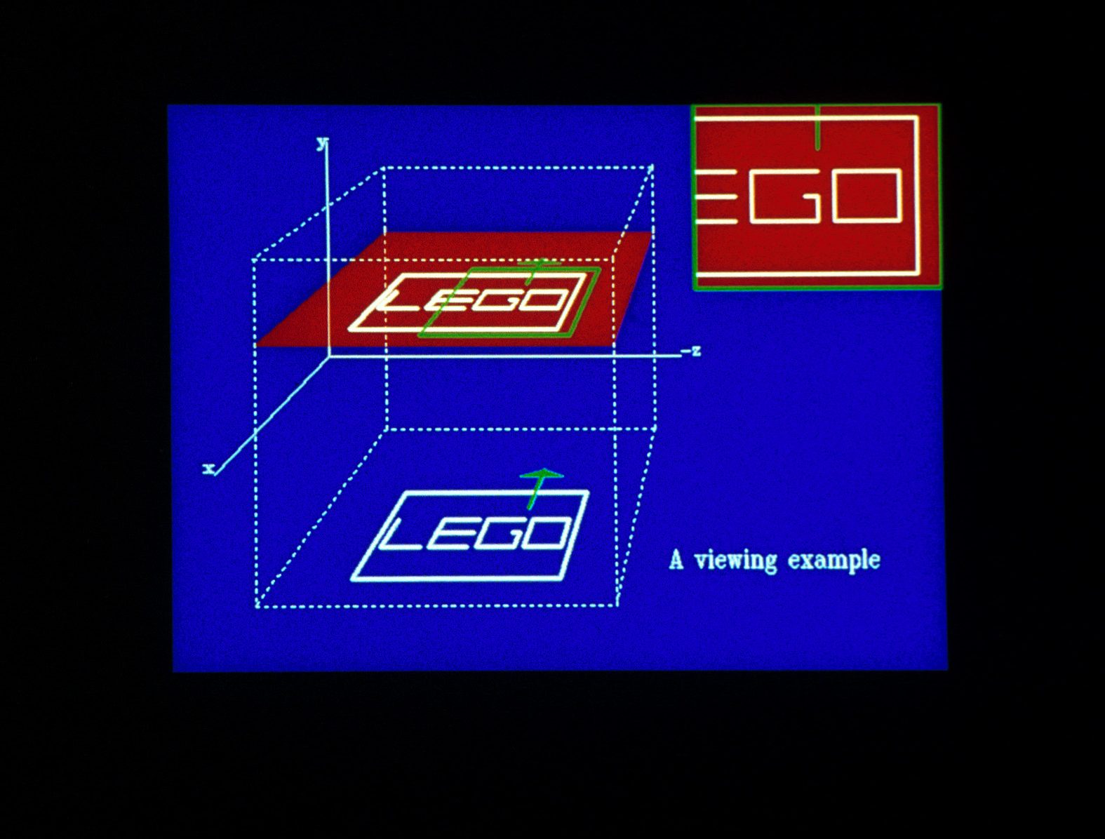
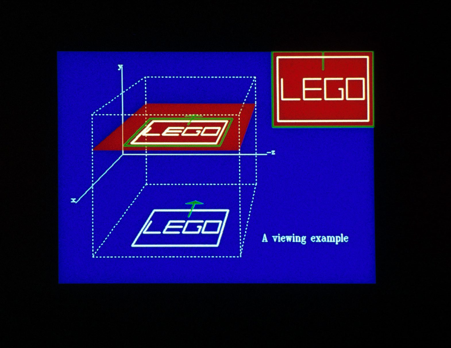
51. Now we apply these notions to properly define the view of the text from slide 44. We define an appropriate view up vector which will determine the direction “up” on the projection plane.
52. Then we need to determine what portion of the view plane should be shown by defining a window in uv-coordinates.
53. By changing the window we can control what part of the object is shown.
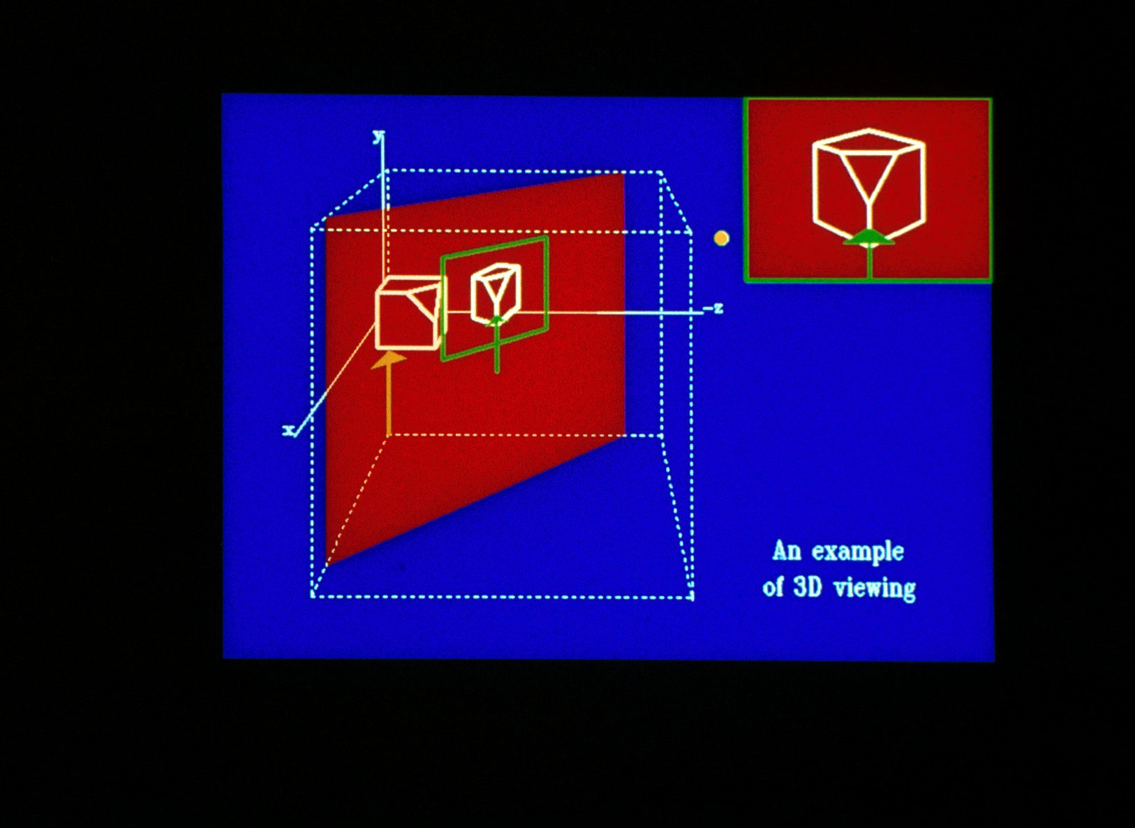
54. Another example of a view specification.
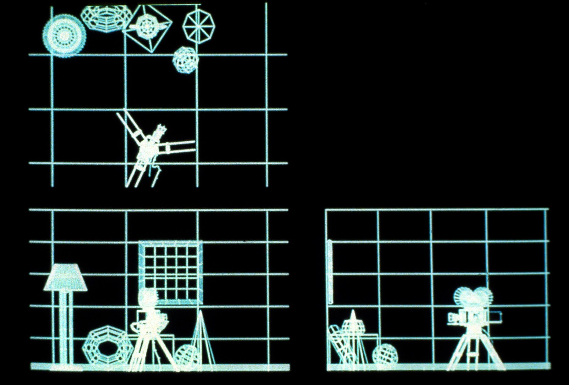
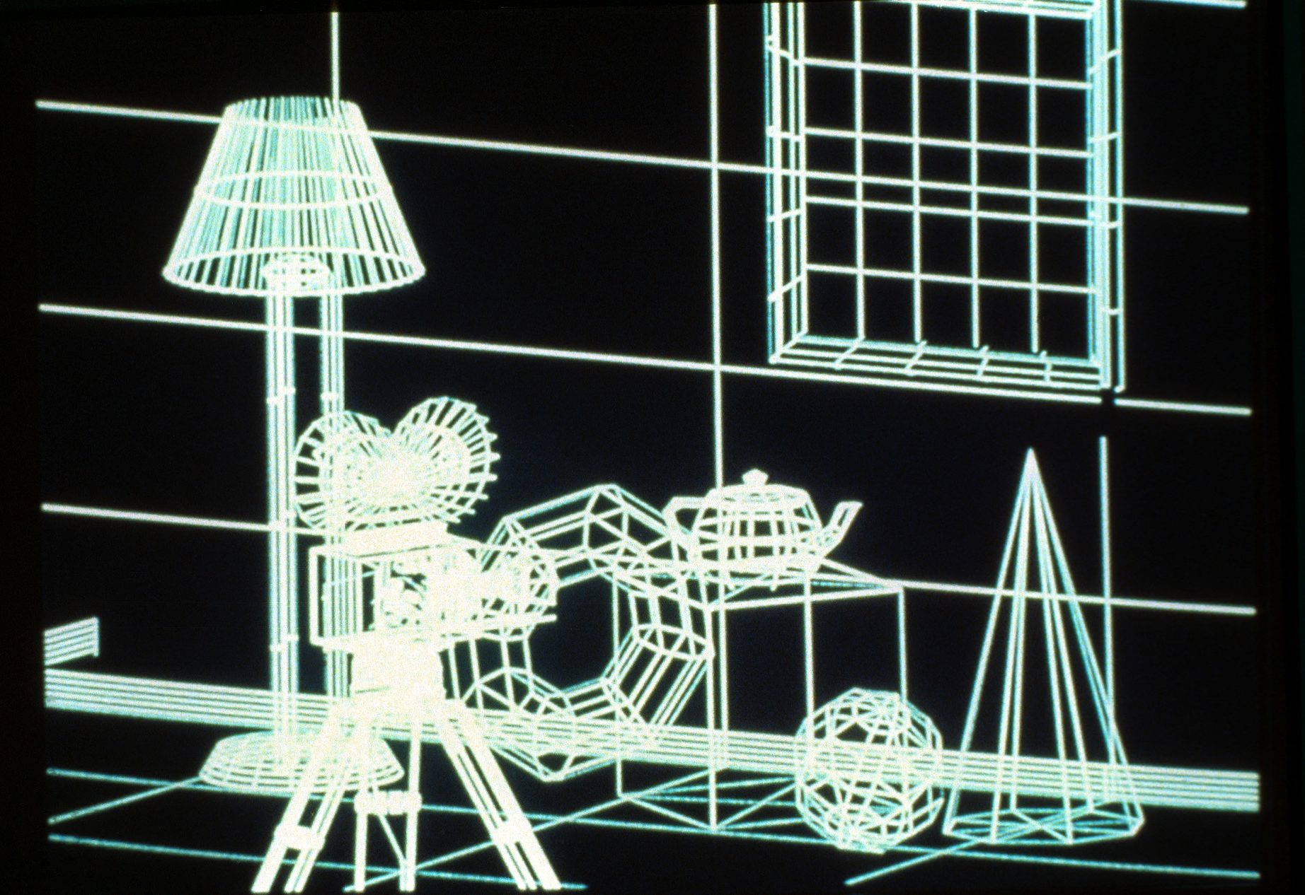
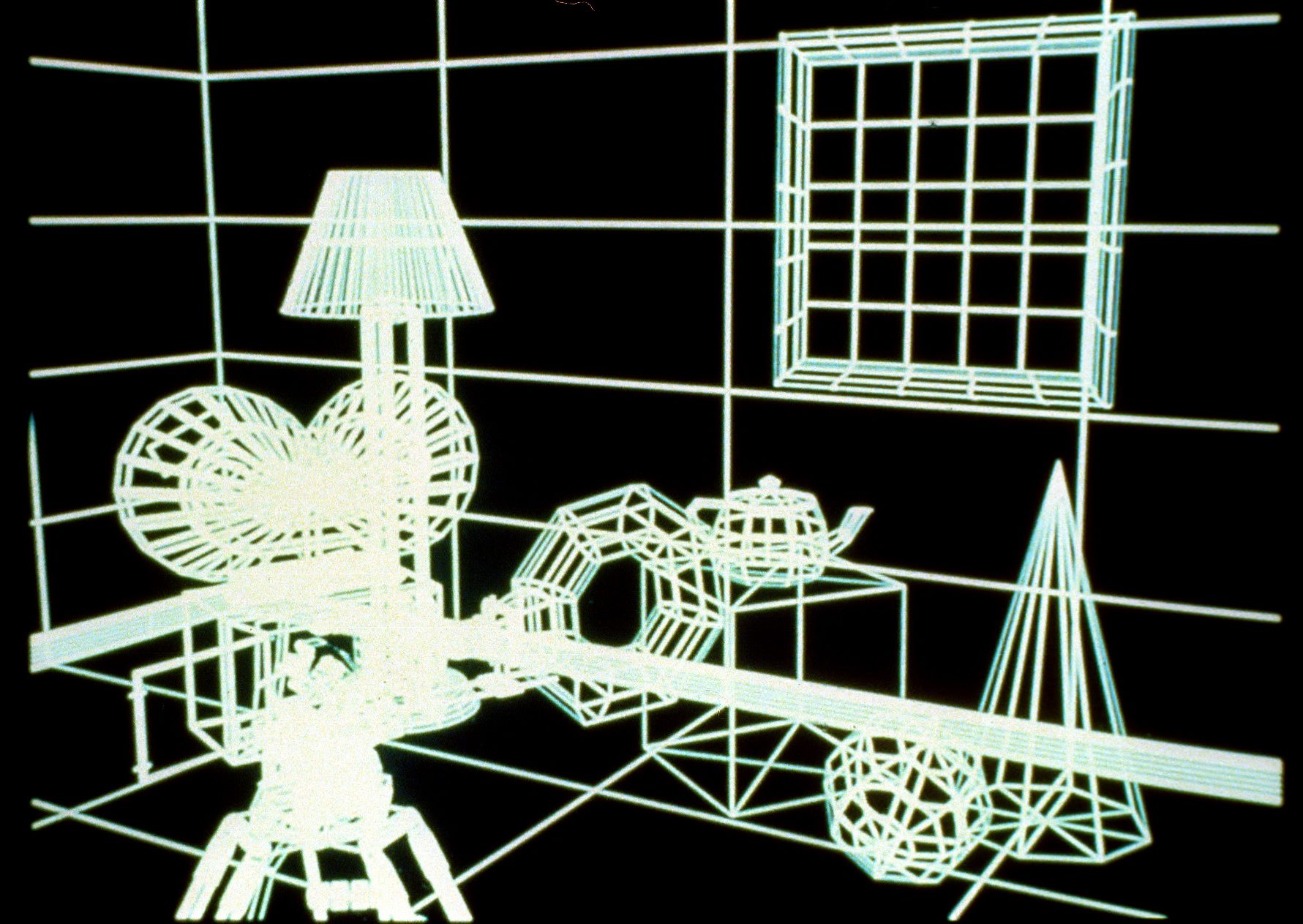
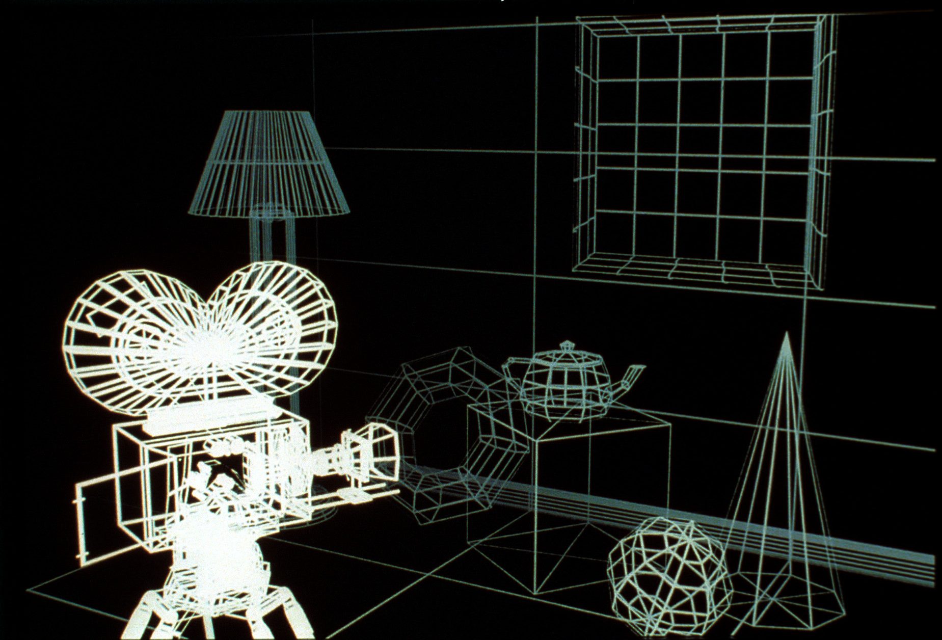
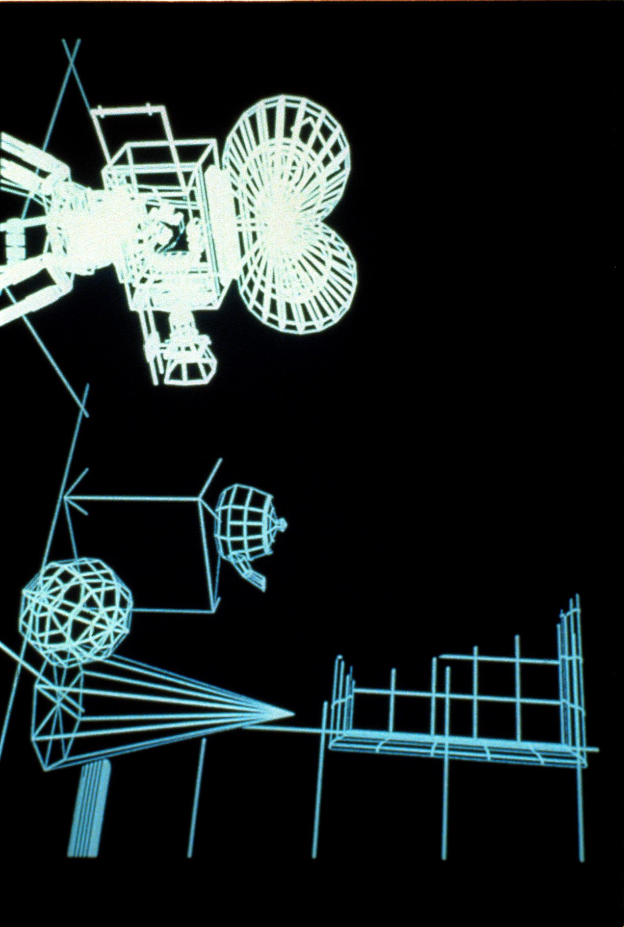
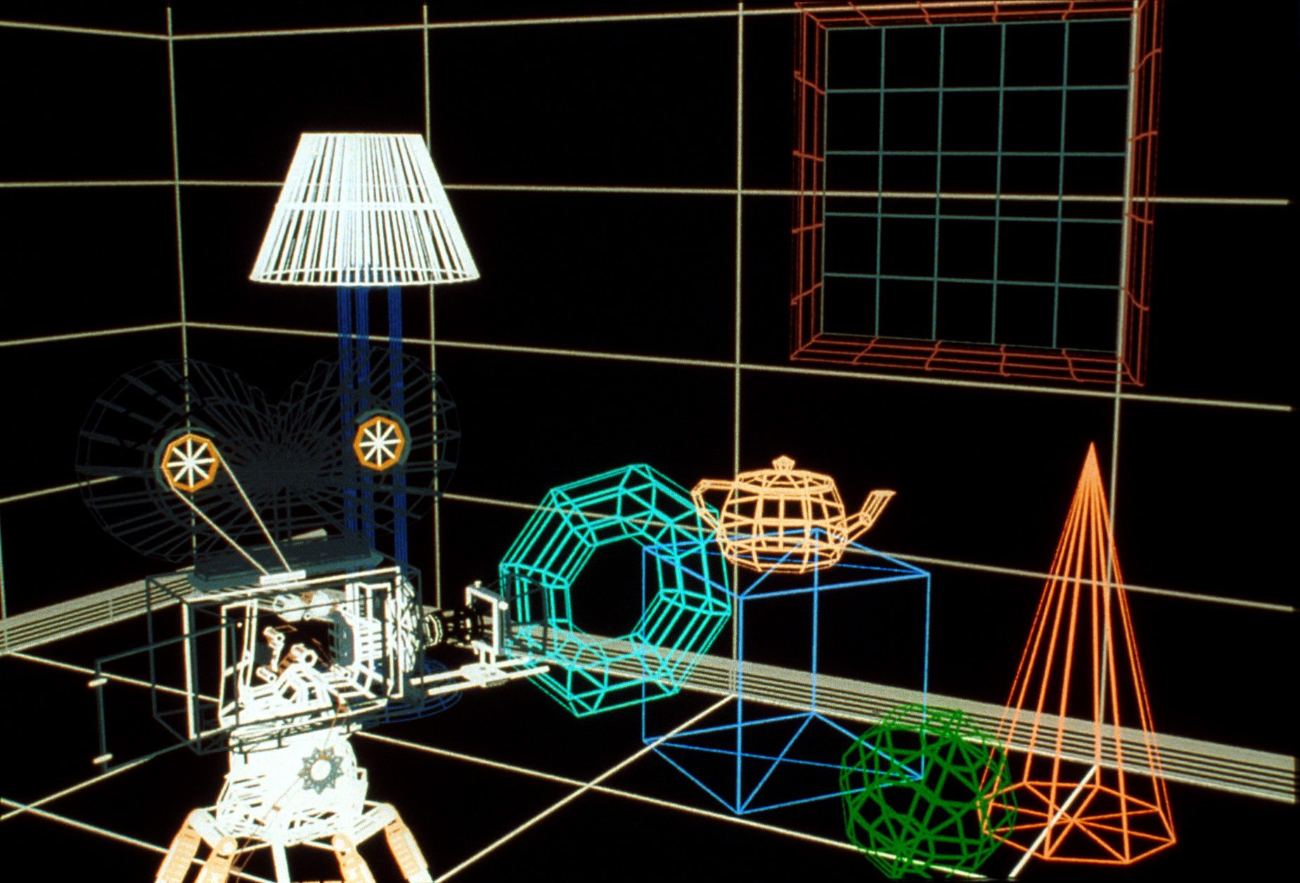
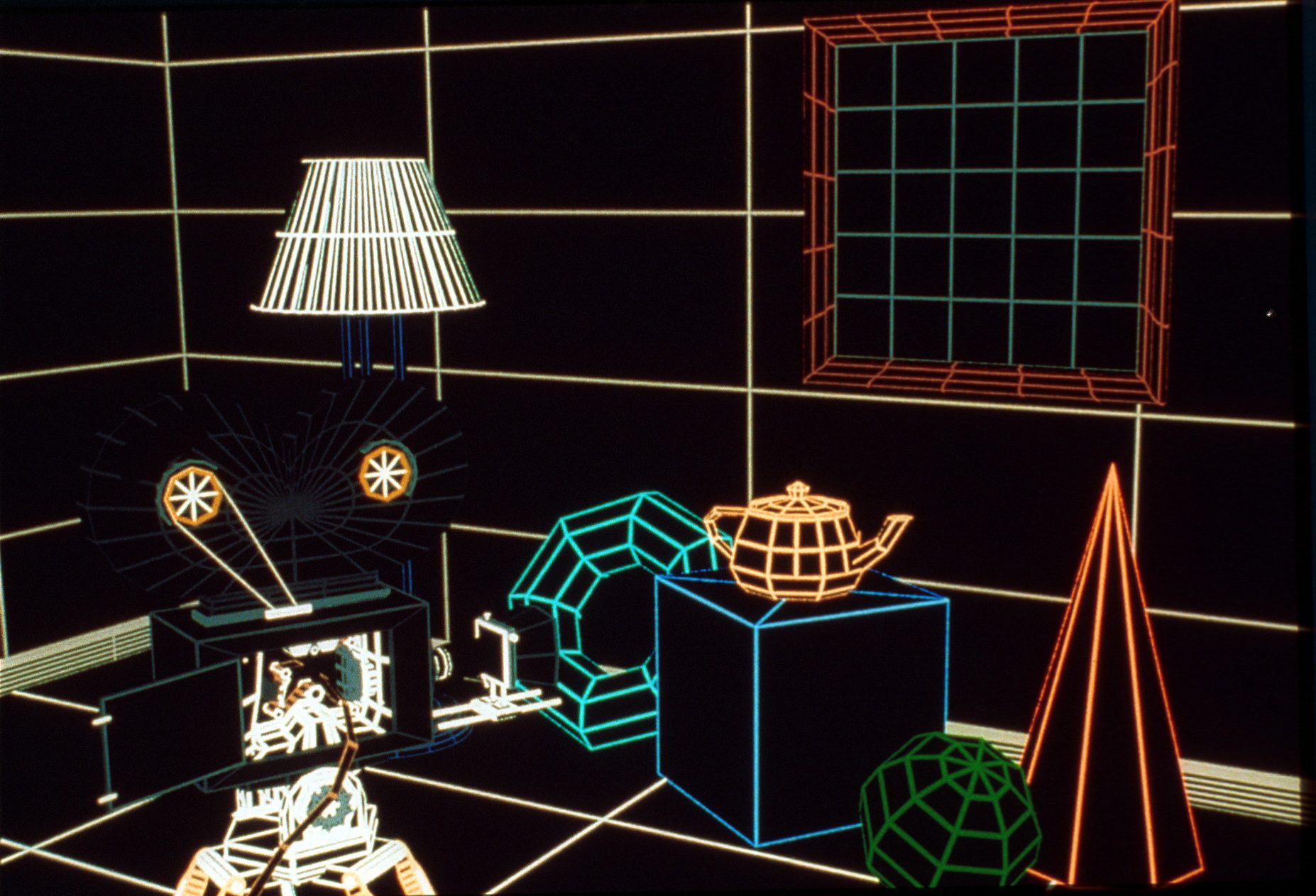
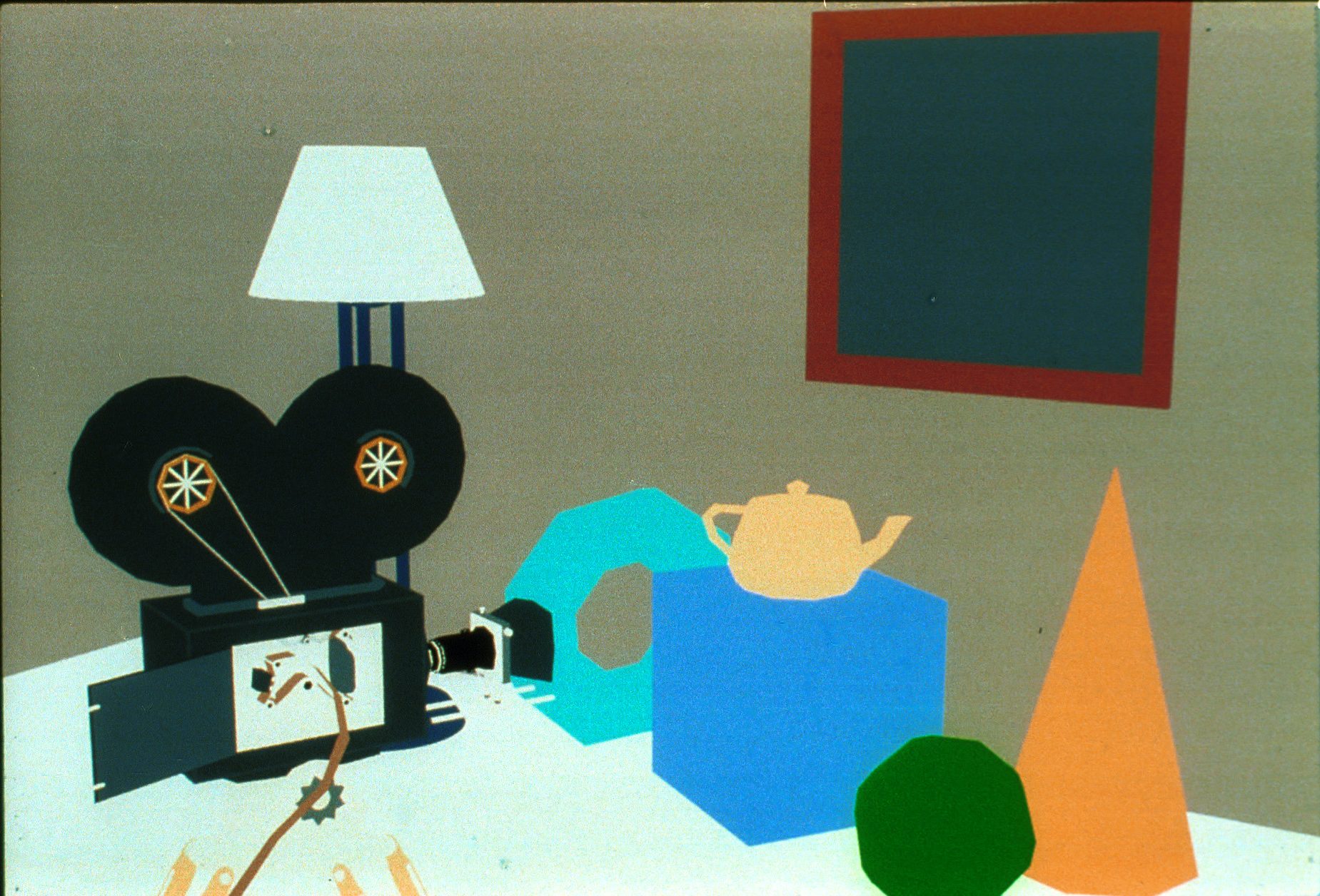
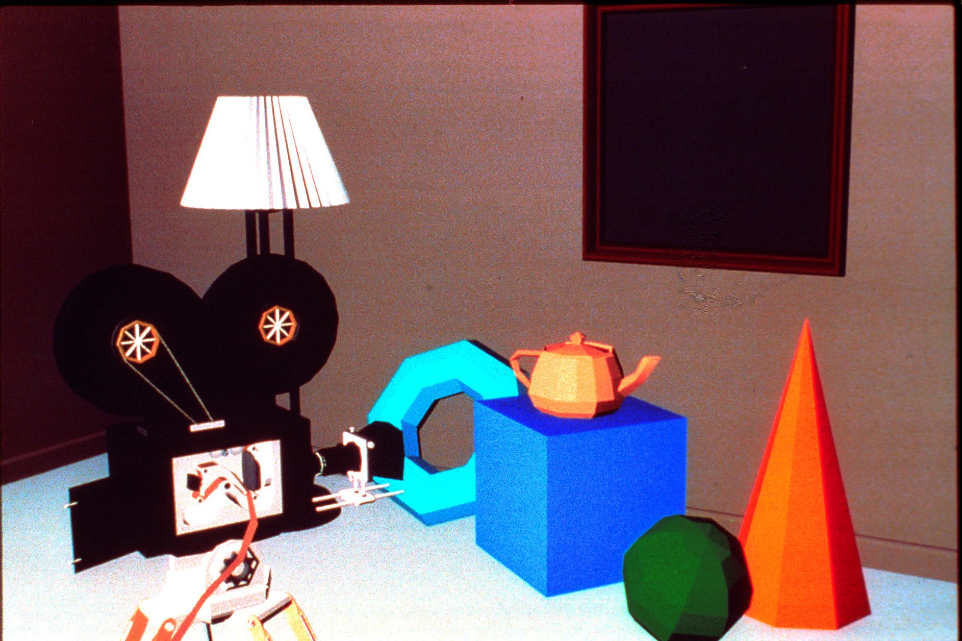
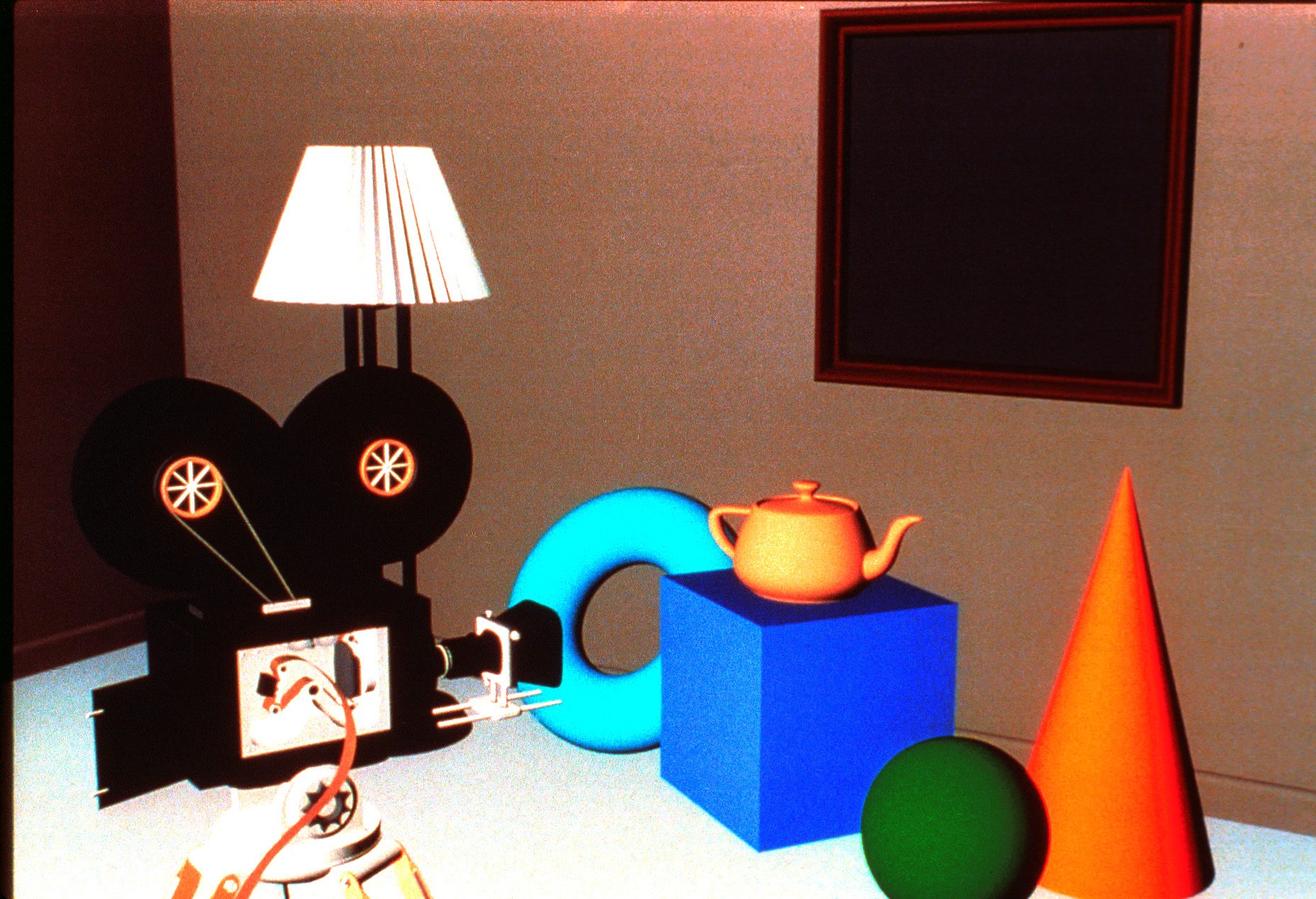
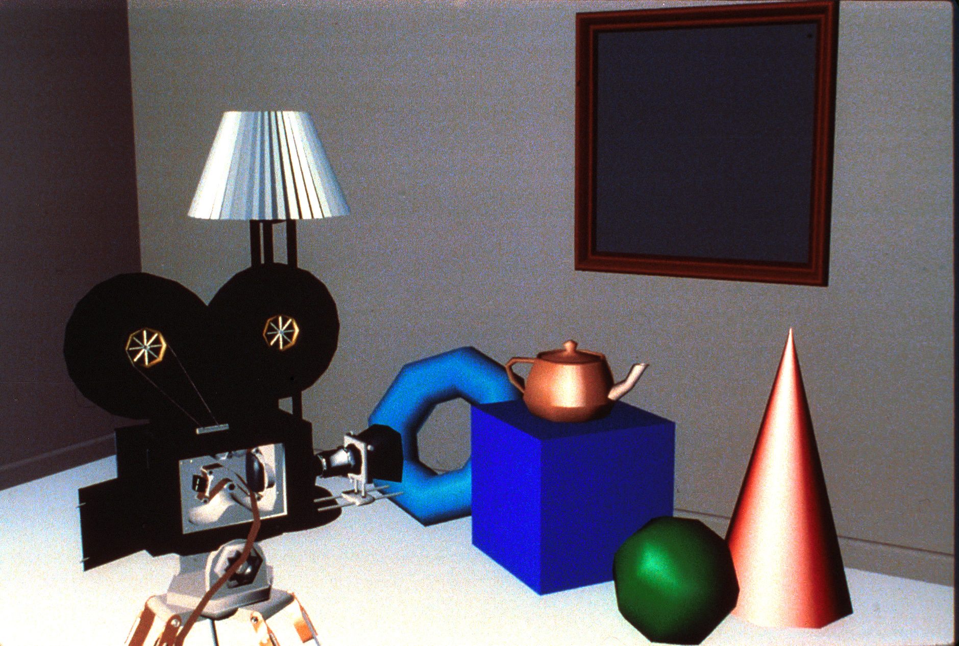
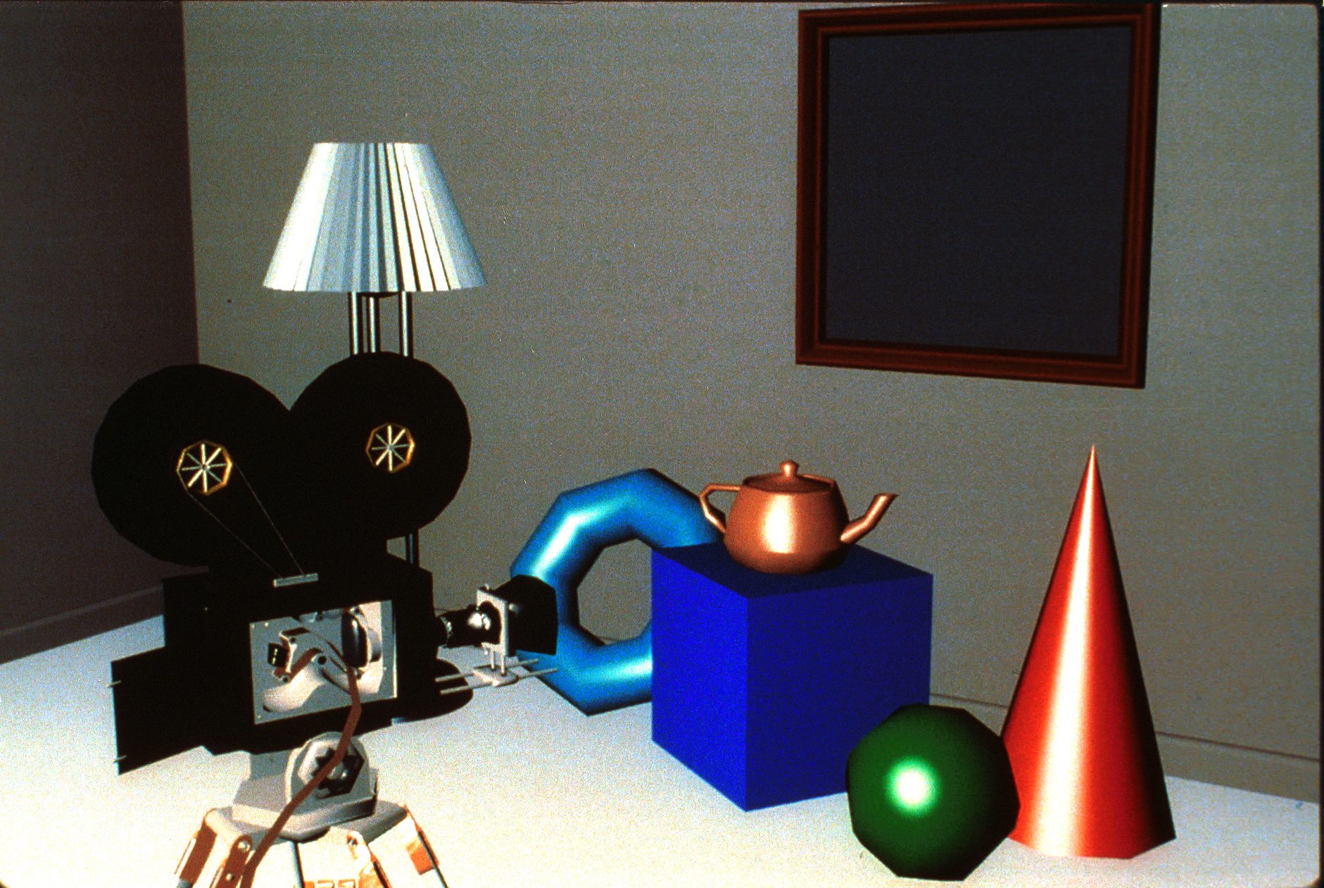
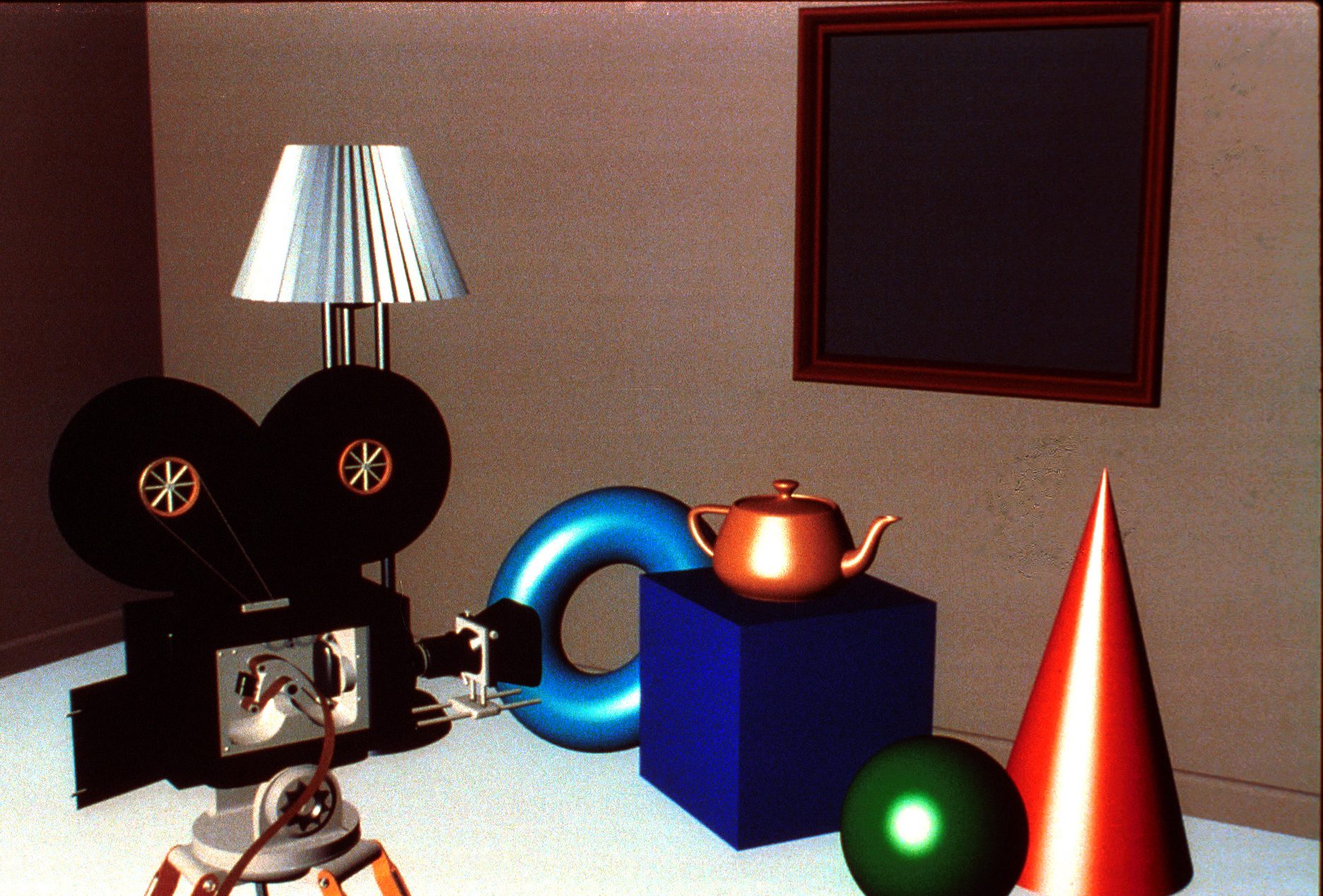
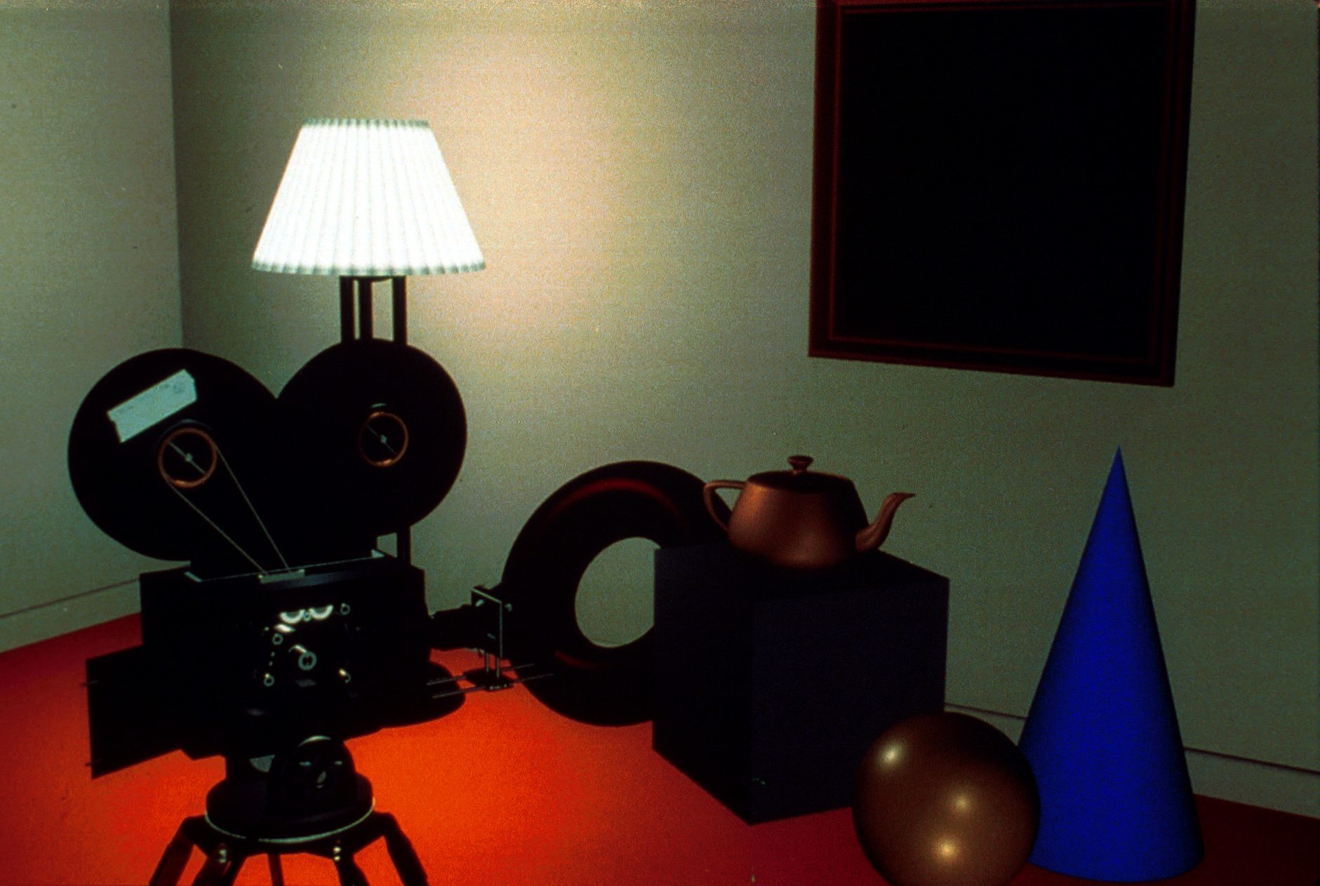
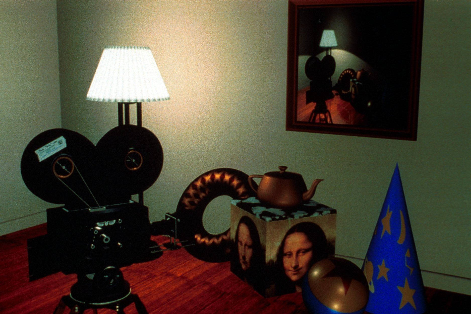
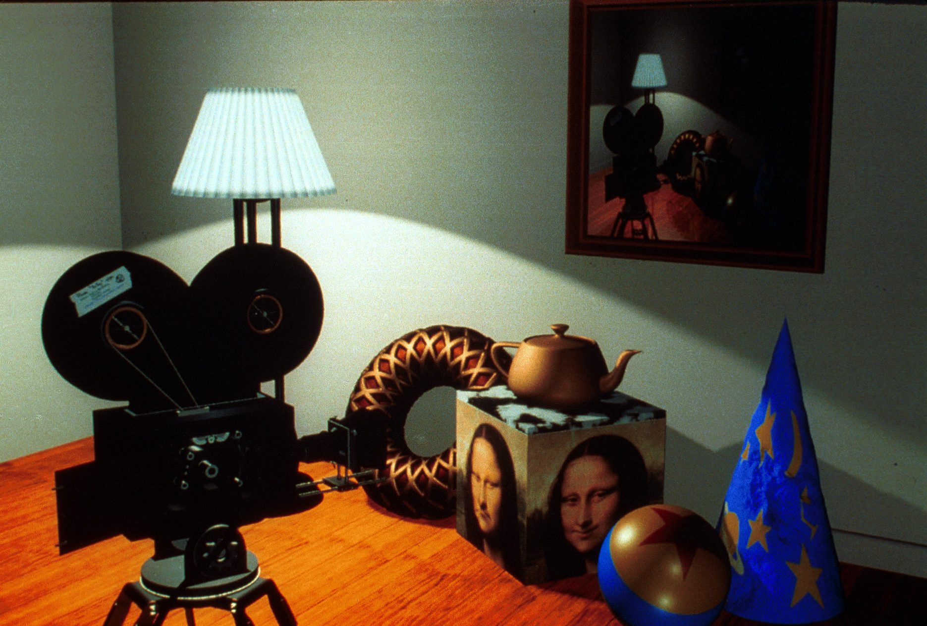
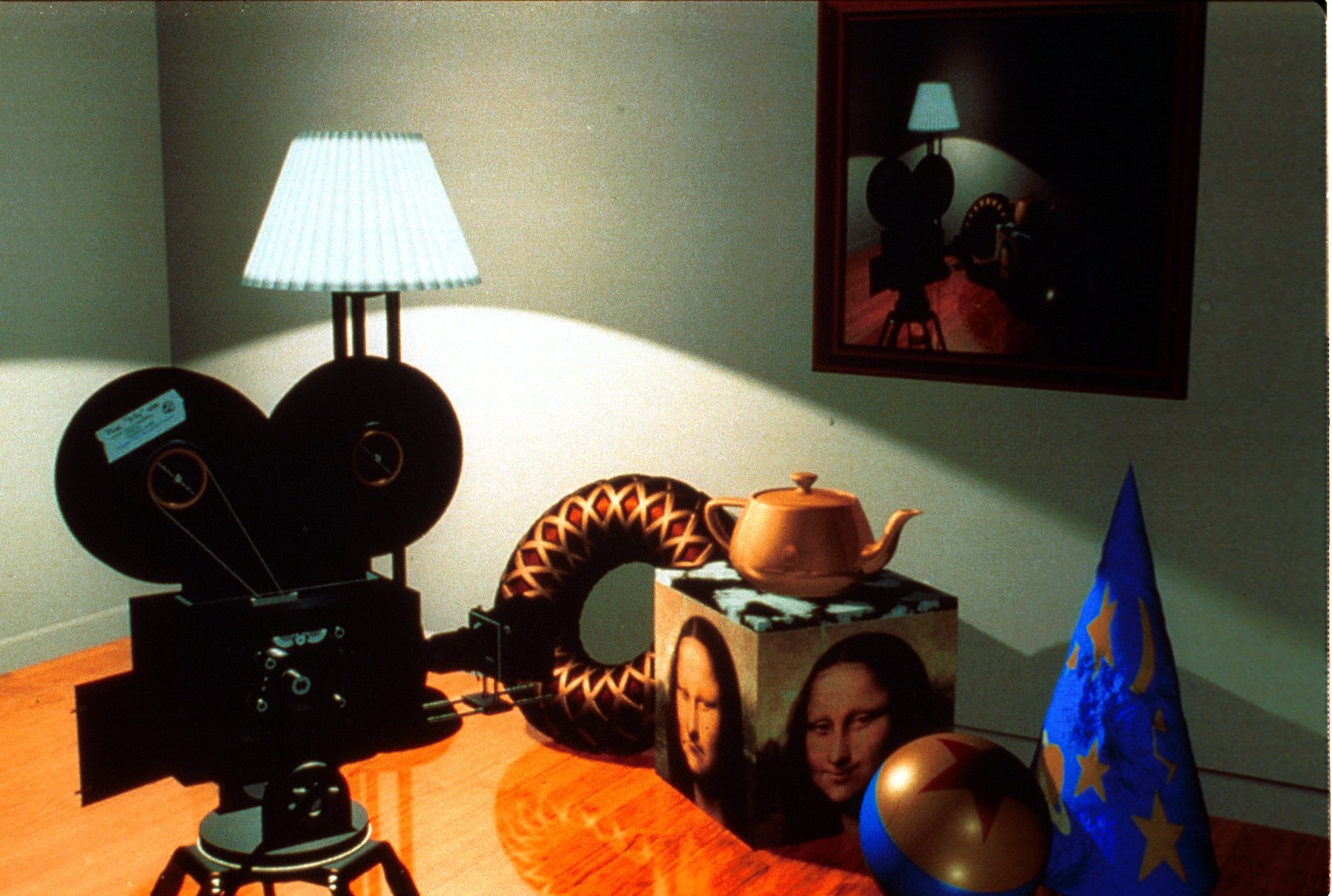
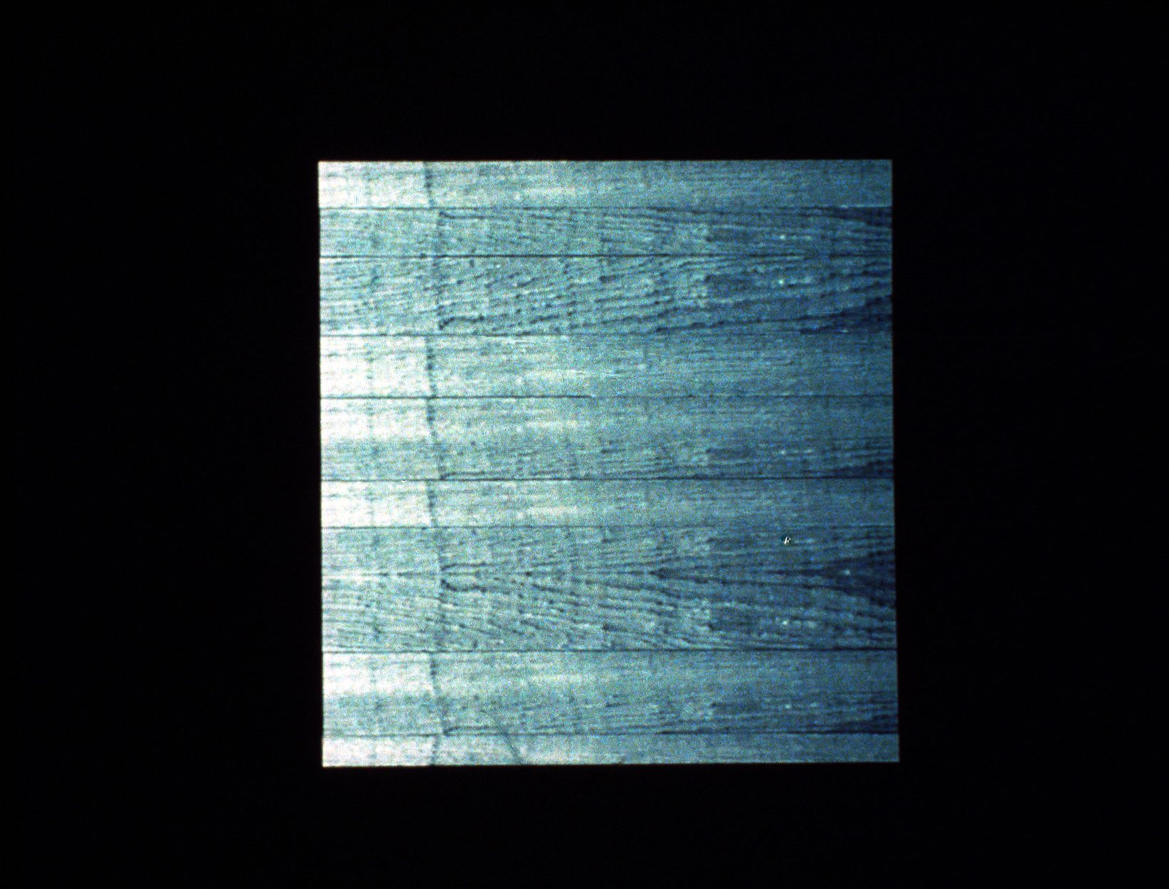
The ShutterBug slide series
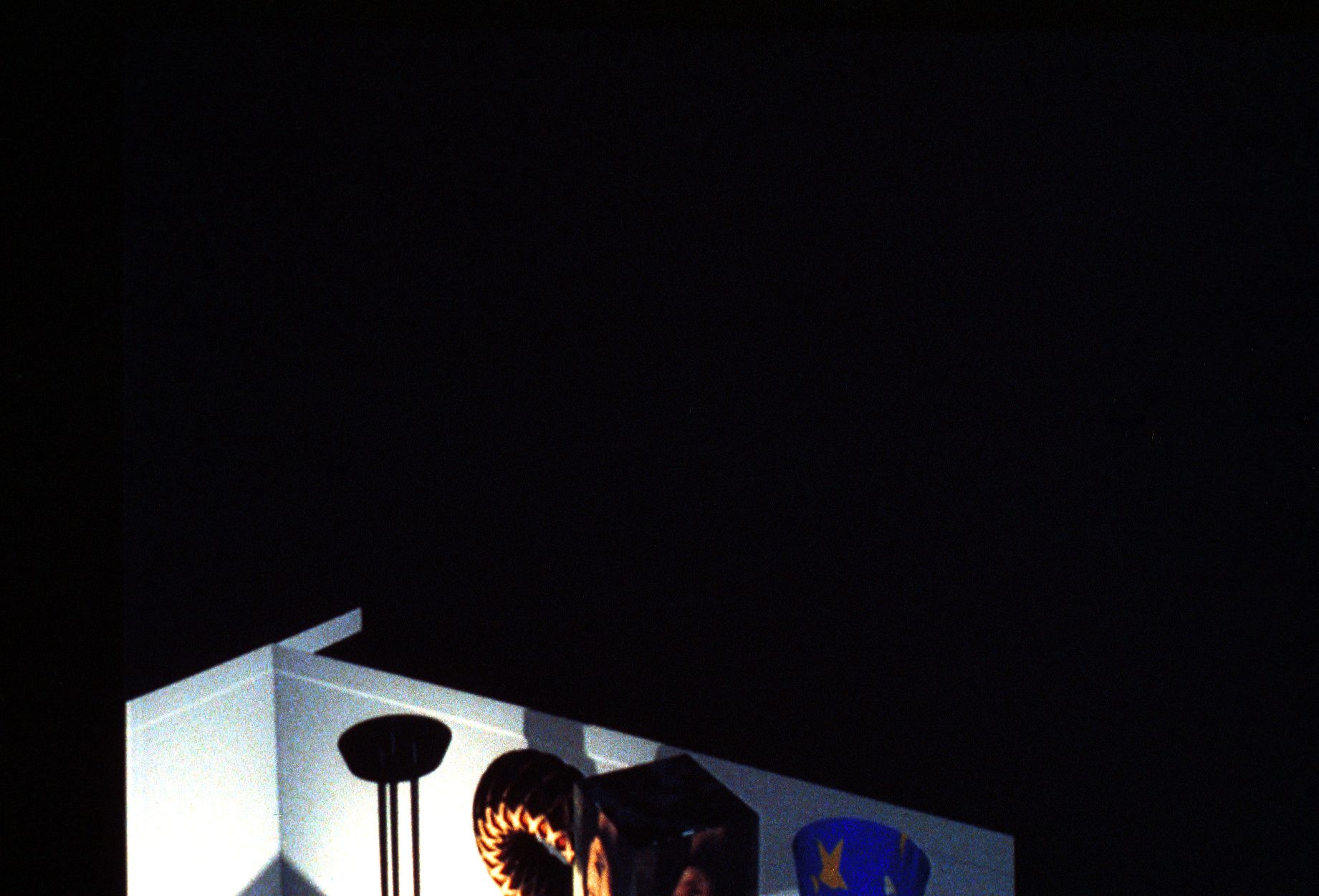
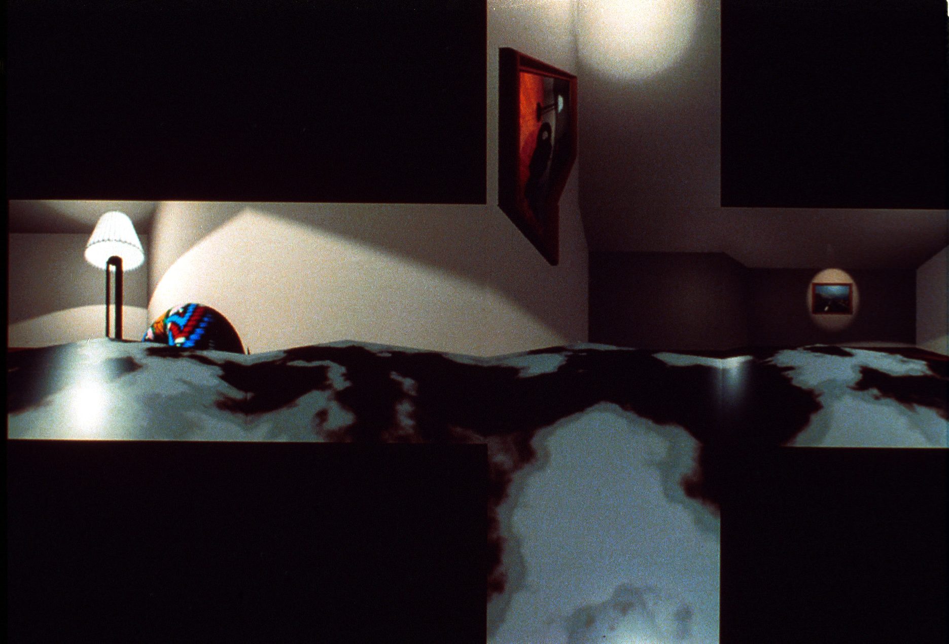
Slides 55 through 78. El Produced by Tom Williams and H.B. Siegel with the assistance of M. W. Mantle, all of Pixar. Copyright 1991, Pixar. This sequence illustrates the progressive refinement of rendering algorithms. The images range from wire frames to photo-realistic renditions including reflections and shadows. The rendering algorithm affects the quality and information conveyed by the image, independent of the underlying three-dimensional model. Following two credits slides, this set includes the 17 slides that are shown in Computer Graphics: Theory and Practice, second edition, by Foley, van Dam, Feiner and Hughes, Addison-Wesley, 1991 as color plates 11.21 through 11.37. The principles these slides illustrate are described in the text and are keyed to the text in the figures’ captions. In addition, the set includes three texture maps, one reflection map and one environment map, respectively, that were used in creating the final image in the series.
Publication Documents:
1991 Education Slide Set Images: