“1993 Education Slide Set”, 1993
Title:
- 1993 Education Slide Set
Year:
- 1993
Conference:
Description:
SIGGRAPH ’93 Educators’ Slide Set Credits
Edited by Rosalee Nerheim-Wolfe
The educators’ slide sets provide high-resolution true-color images to support the teaching of computer graphics as art and as computer science. The 1993 set presents several computer graphics algorithms and visualizes their effects. Topics include drawing lines and circles, aliasing and antialiasing, and examining radiosity. can be obtained via anonymous ftp on siggraph.org. The explanatory material is available as ASCII text (txt), Rich Text format (rtf) and PostScript (ps): Toby Howard developed drawing lines and circles and contributed to the antialiasing section. David Abramoske and Cindi Gryniewicz created the raytraced images for the antialiasing section. Jenny Morlan served as art director for both of the first two sections. The Ohio State University Advanced Computing Center for the Arts and Design, including Stephen Spencer and Wayne Carlson, created the section on radiosity.
/publications/proceedings/siggraph93/slidesets/txt/educators.txt /publications/proceedings/siggraph93/slidesets/rtf/educators.rtf /publications/proceedings/siggraph93/slidesets/ps/educators.ps
The full color 35mm slide set containing 78 slides can be Accompanying the slide set is a booklet that contains explanatory material. The booklet is packaged with the slide set, but ordered from: ACM order department, P.O. Box 64145, Baltimore, MD 21264; 1-800-342-6626. The ACM order number for the SIGGRAPH ’93 educators’ slide set is 915932. The cost is $33 for members; $44 for non-members. A brief description of the three parts of this set follows.
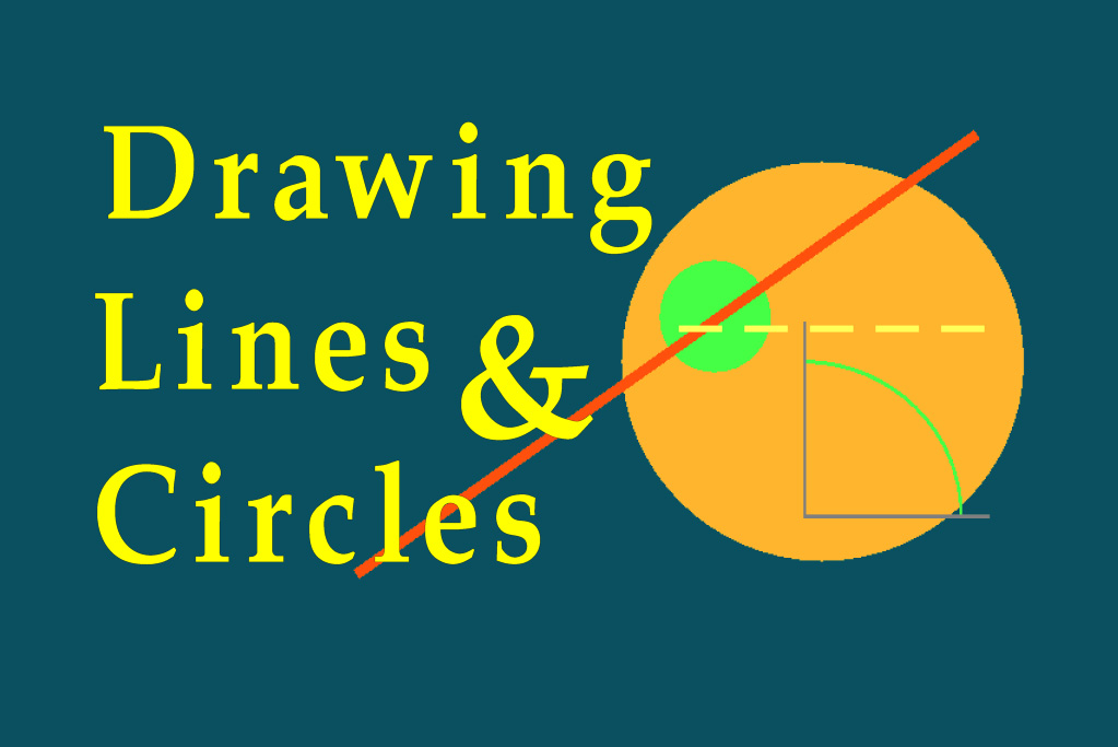
Drawing Lines and Circles Slides 2 – 27 This section illustrates the basic principles of scan-converting lines and circles for raster displays. Scan-conversion is the process of determining which pixels should be illuminated in order to display a representation of a geometrical object which is as faithful as possible to the exact continuous geometry of the object.
2 – Title slide
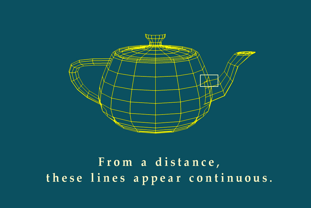
3 – Lines of a display screen
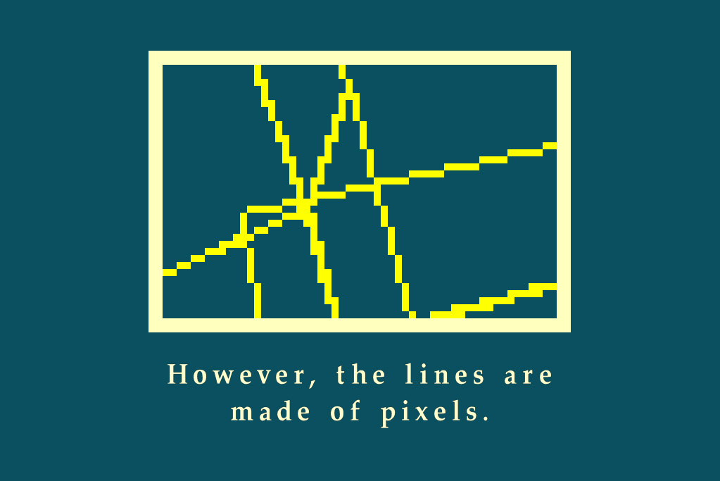
4 – Lines as pixels
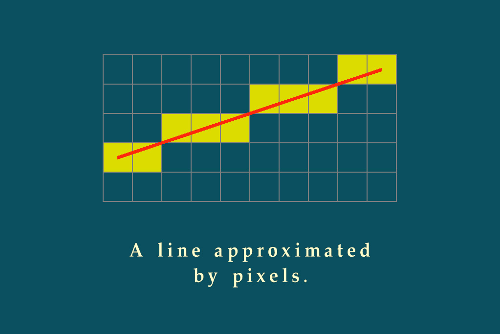
5 – Approximating a line with pixels
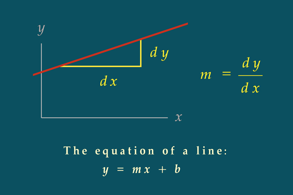
6 – The equation of a line
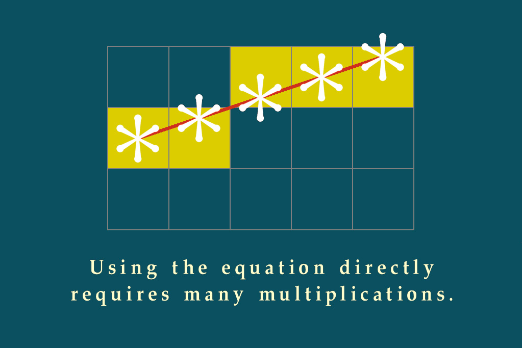
7 – Brute force scan conversion
8 – The DDA algorithm
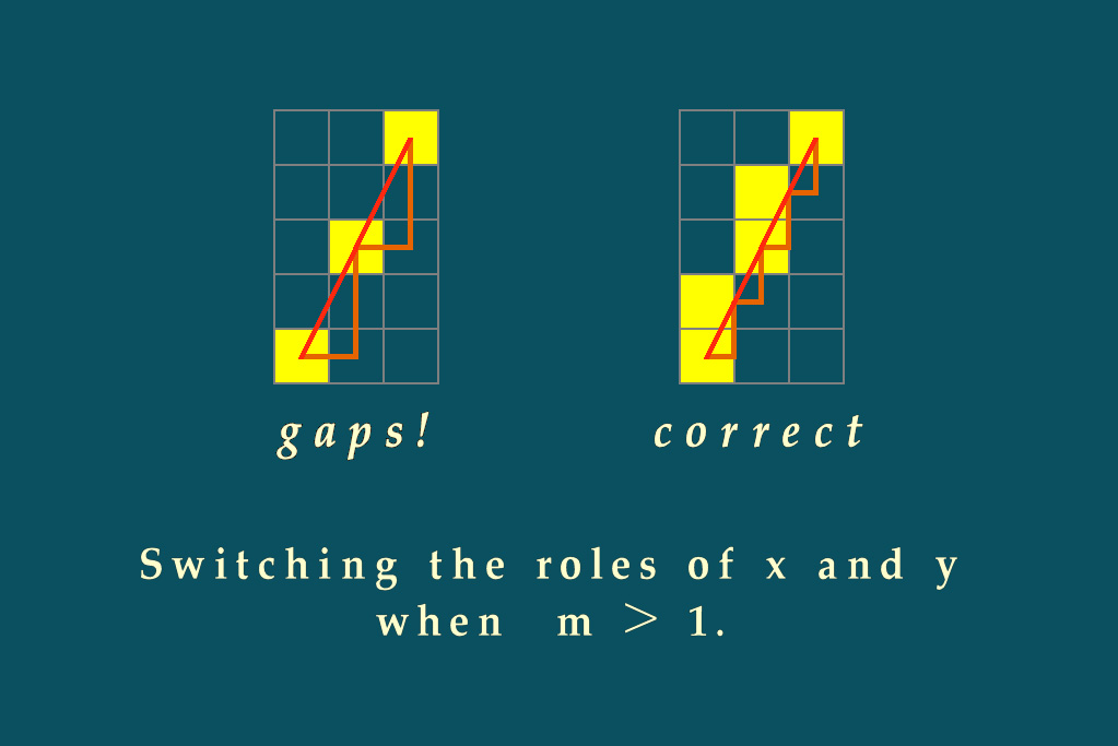
9 – The DDA algorithm for lines with -I < m < 1
10 – Gaps occur when m > l
11 – Bresenham’s algorithm
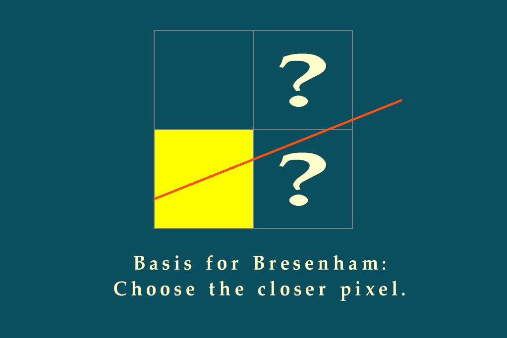
12 – Choosing between two pixels
13 – Finding the closer pixel
14 – Another example
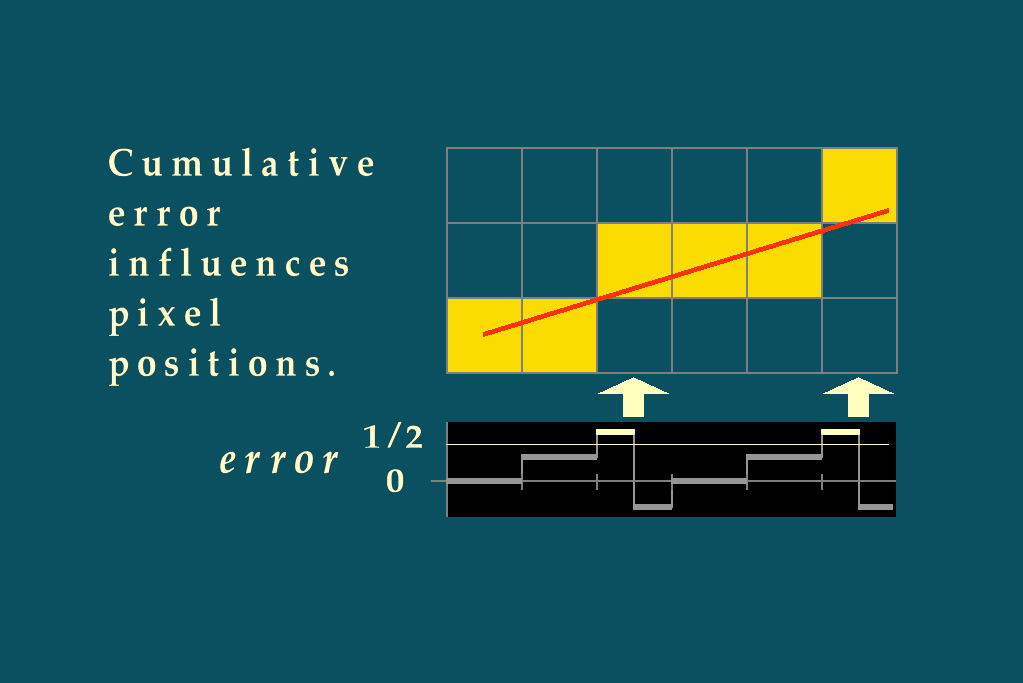
15 – Introducing an error term
16 – Using the error term
17 – The error term is fractional
18 – Rewriting the error term
19 – Using the integer scaled error term
20 – Scan-converting circles
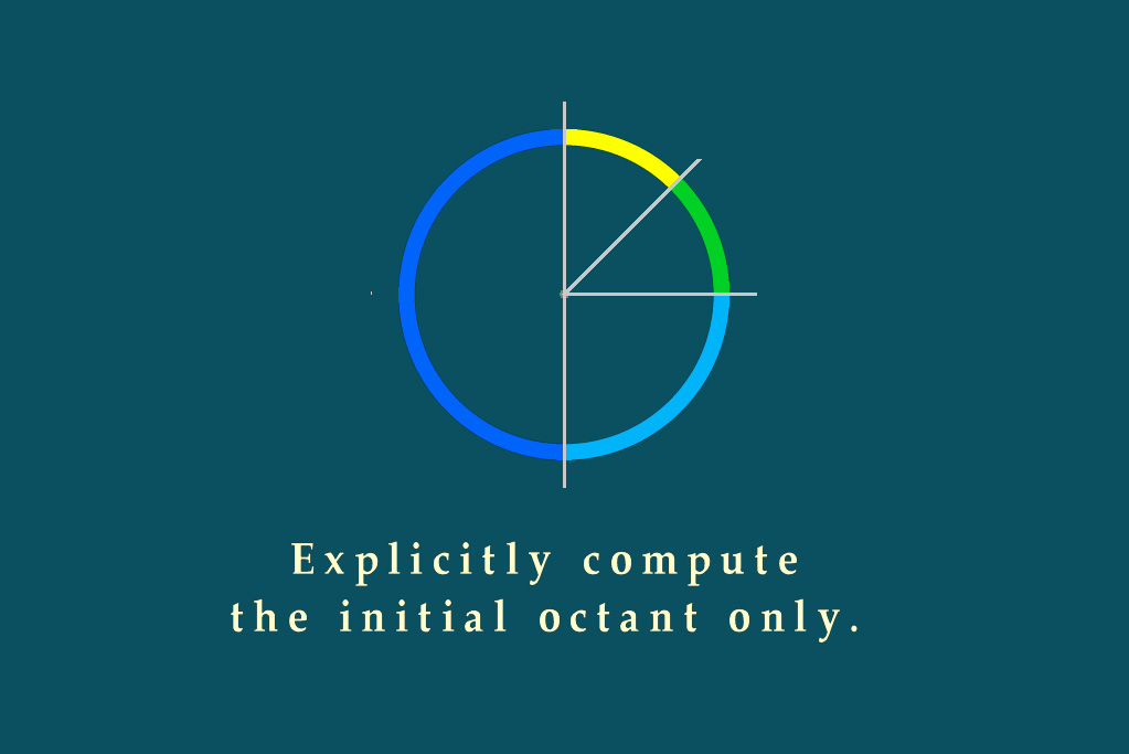
21 – The eight-fold symmetry of the circle
22 – Computing the initial octant
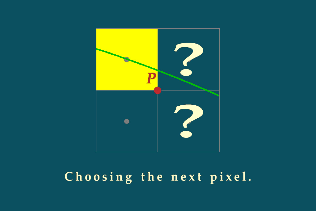
23 – Choosing the next pixel
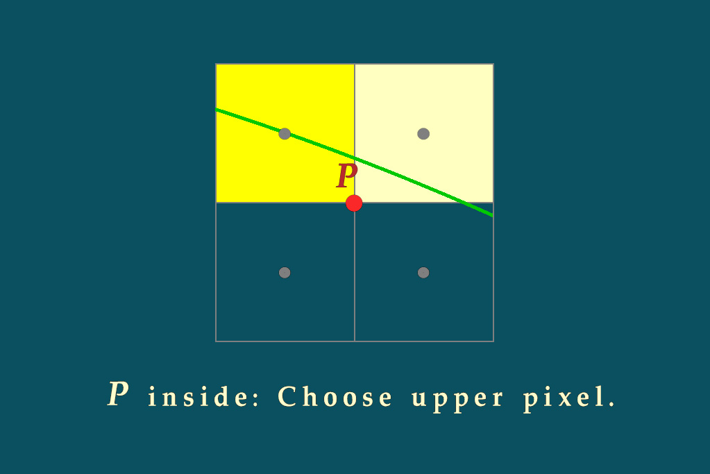
24 – Using a reference point P
25 – P is outside the circle
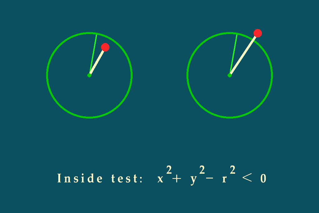
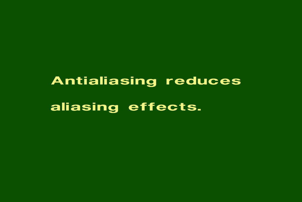
26 – Determining if a point lies inside a circle
27 – Credits Aliasing and Antialiasing
Slides 28 – 52 This section of the slide set will demonstrate how aliasing affects the rendering of images, and how antialiasing methods can soften or reduce the effects of aliasing.
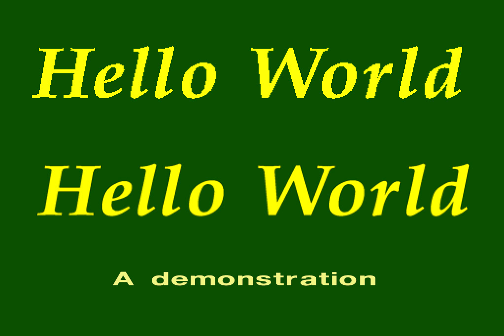
28 – Title slide
29 – Aliasing
30 – Original scene
31 – Sampling the scene
32 – Rendered image
33 – Effects caused by aliasing
34 – Jagged profiles
35 – Improperly rendered detail
36 – Disintegrating textures
37 – Antialiasing
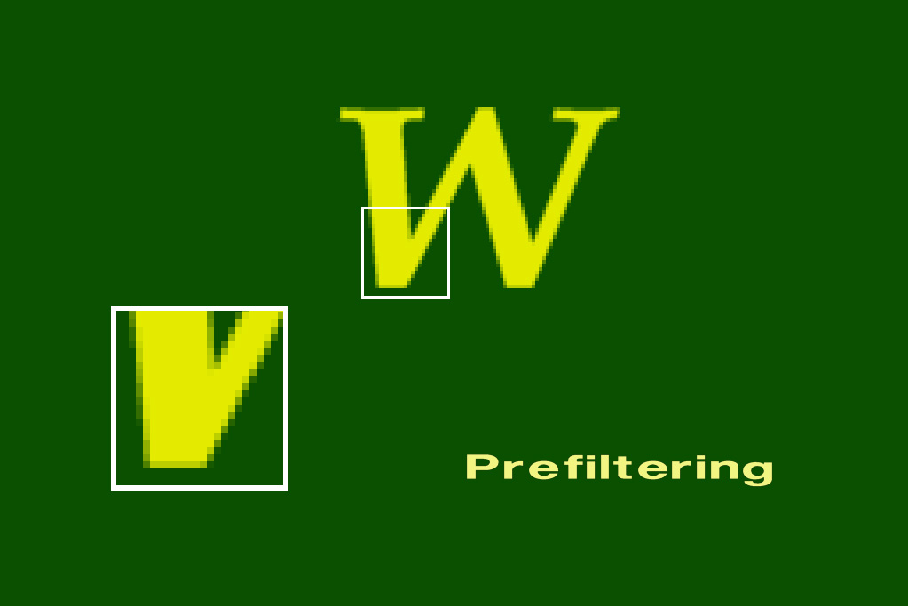
38 – Prefiltering
39 – Basis for prefiltering algorithms
40 – Prefiltering Demonstration
41 – Closeup
42 – Closeup of prefiltered Image
43 – Postfiltering
44 – Sampling in the postfiltering method
45 – Filters
46 -Using a filter to compute a pixel’s color
47 – Student work
48 – No antialiasing
49 – 3×3 supersampling, 3×3 unweighted filter
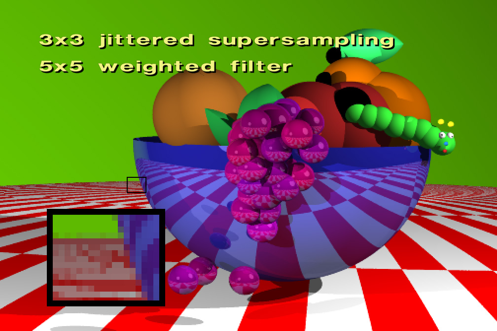
50 – 3×3 supersampling, 5×5 weighted filter
51 – 3×3 supersampling, jittered samples, 3×3 weighted filter
52 – Credits Examining Radiosity
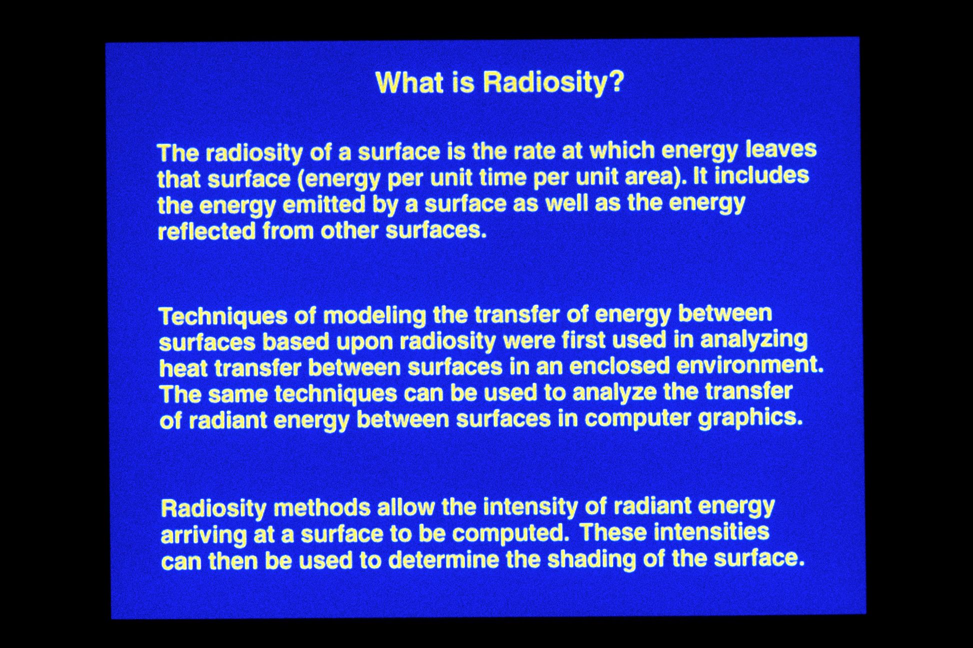
Slides 53 – 78 This section describes an approach to generating computer graphics based on the concept of energy transfer between surfaces. This approach is commonly known as radiosity. We first describe the basic algorithm, and then cover extensions to it. For this method of image generation, we make some basic assumptions. We treat the scene being rendered as a closed environment containing a number of surfaces. A surface may be a source of illum.ination (a light), or an object which reflects light. To create an image of the scene we consider the exchange of light energy between all the objects in the closed environment.
53 – Title slide
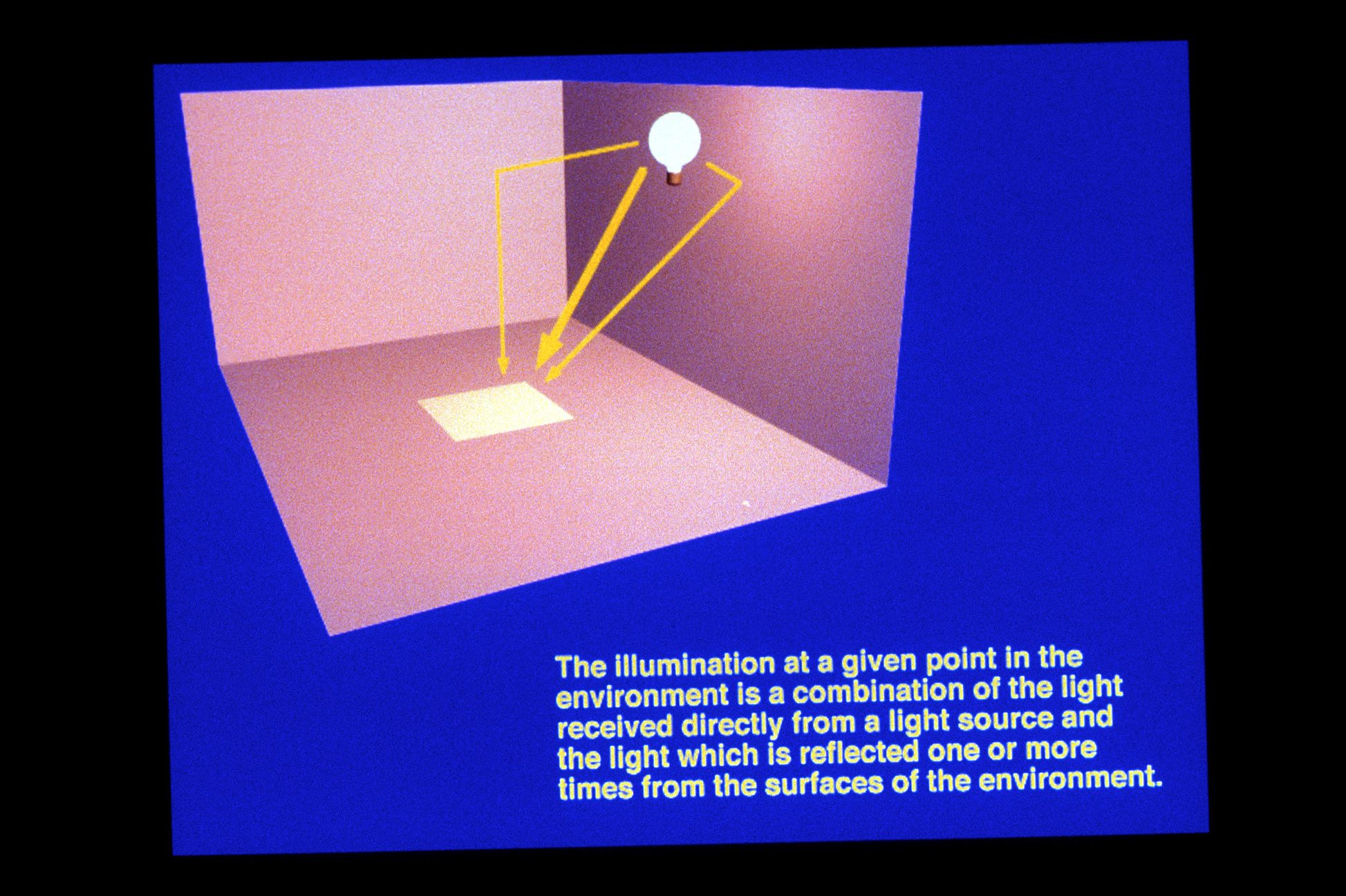
54 – Direct and indirect light
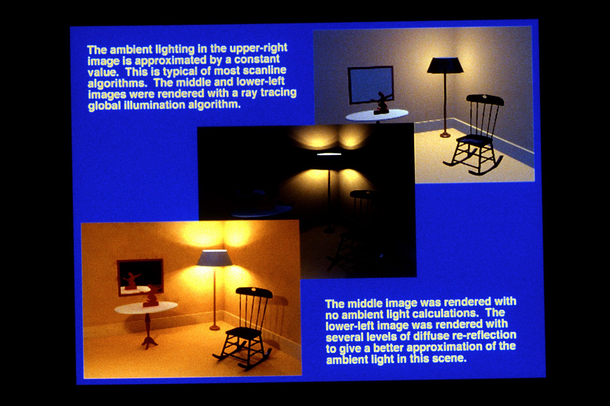
55 – Examples of rendering methods
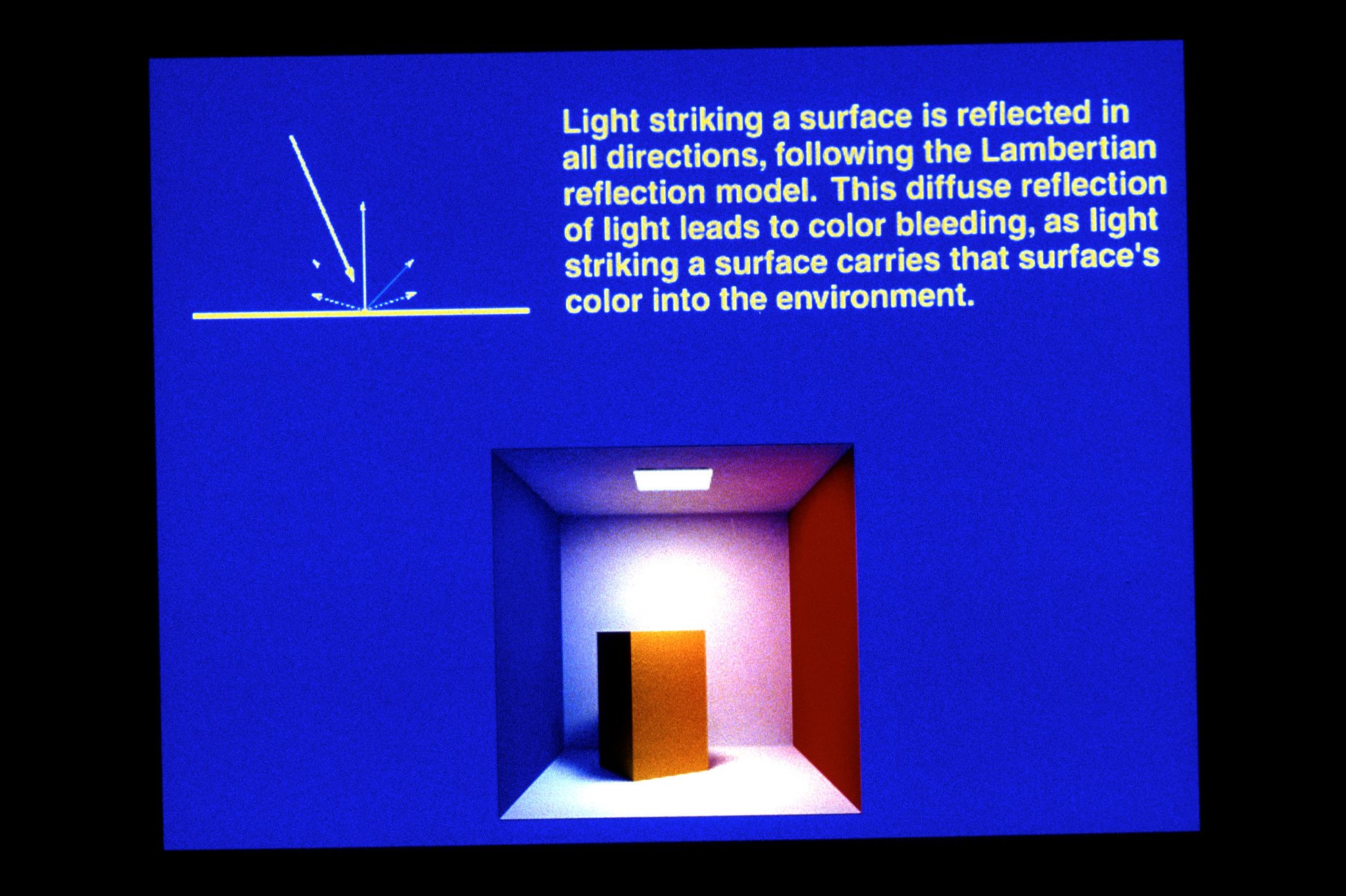
56 – Diffuse interreflection
57 – Introduction to radiosity
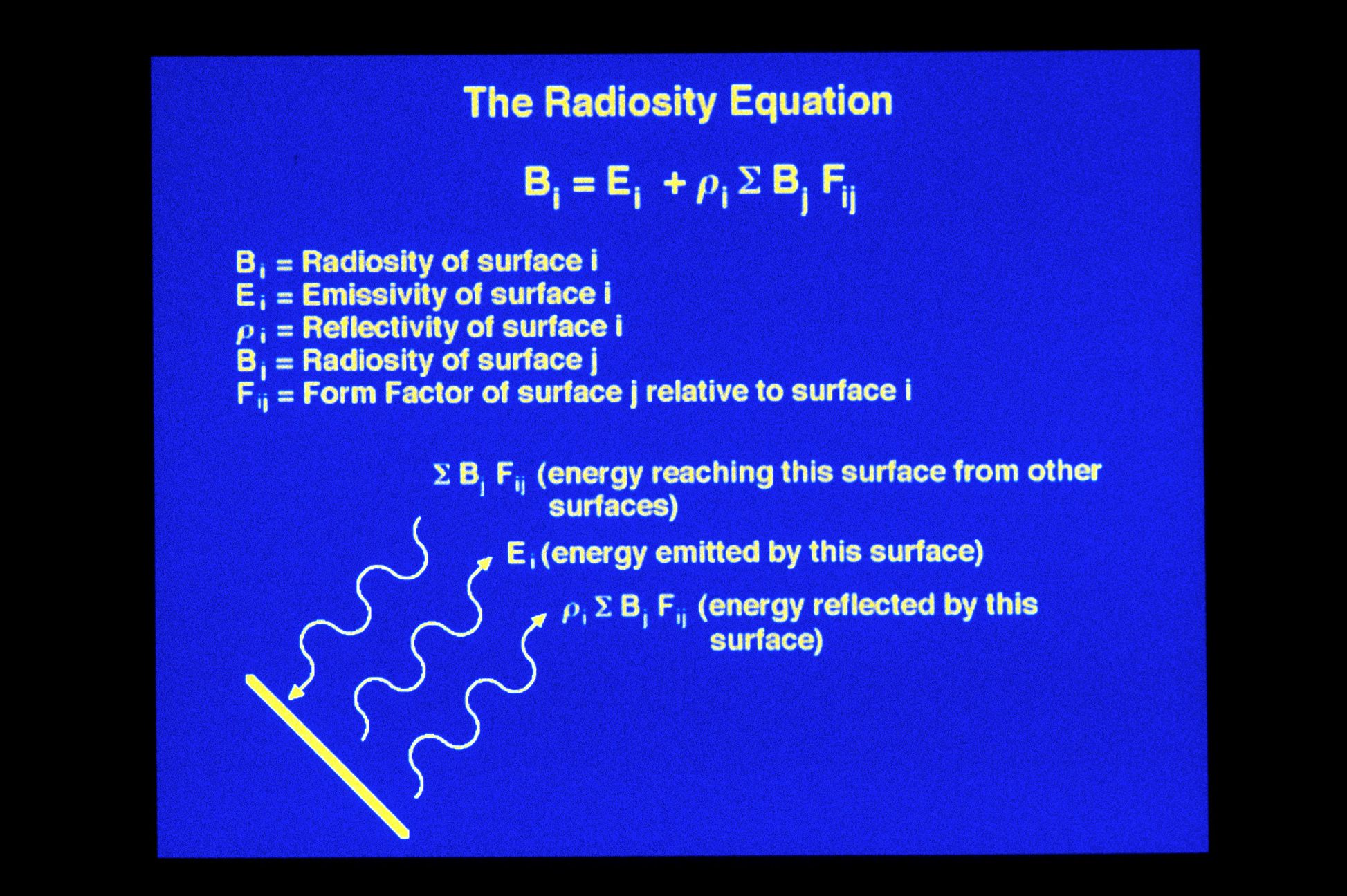
58 – The radiosity equation
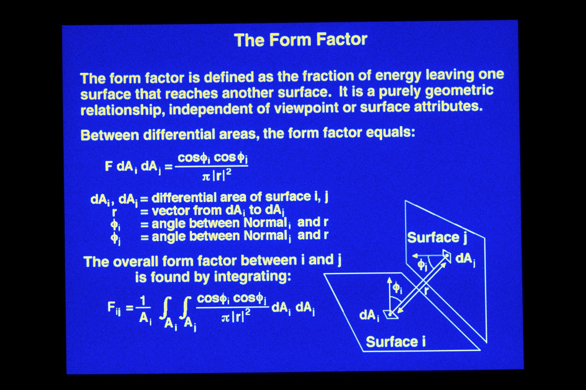
59 – The form factor
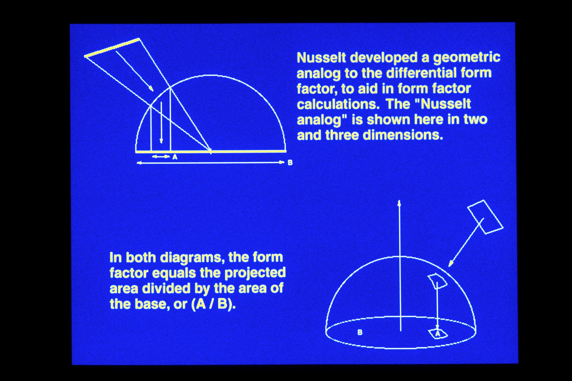
60 – The Nusselt analog
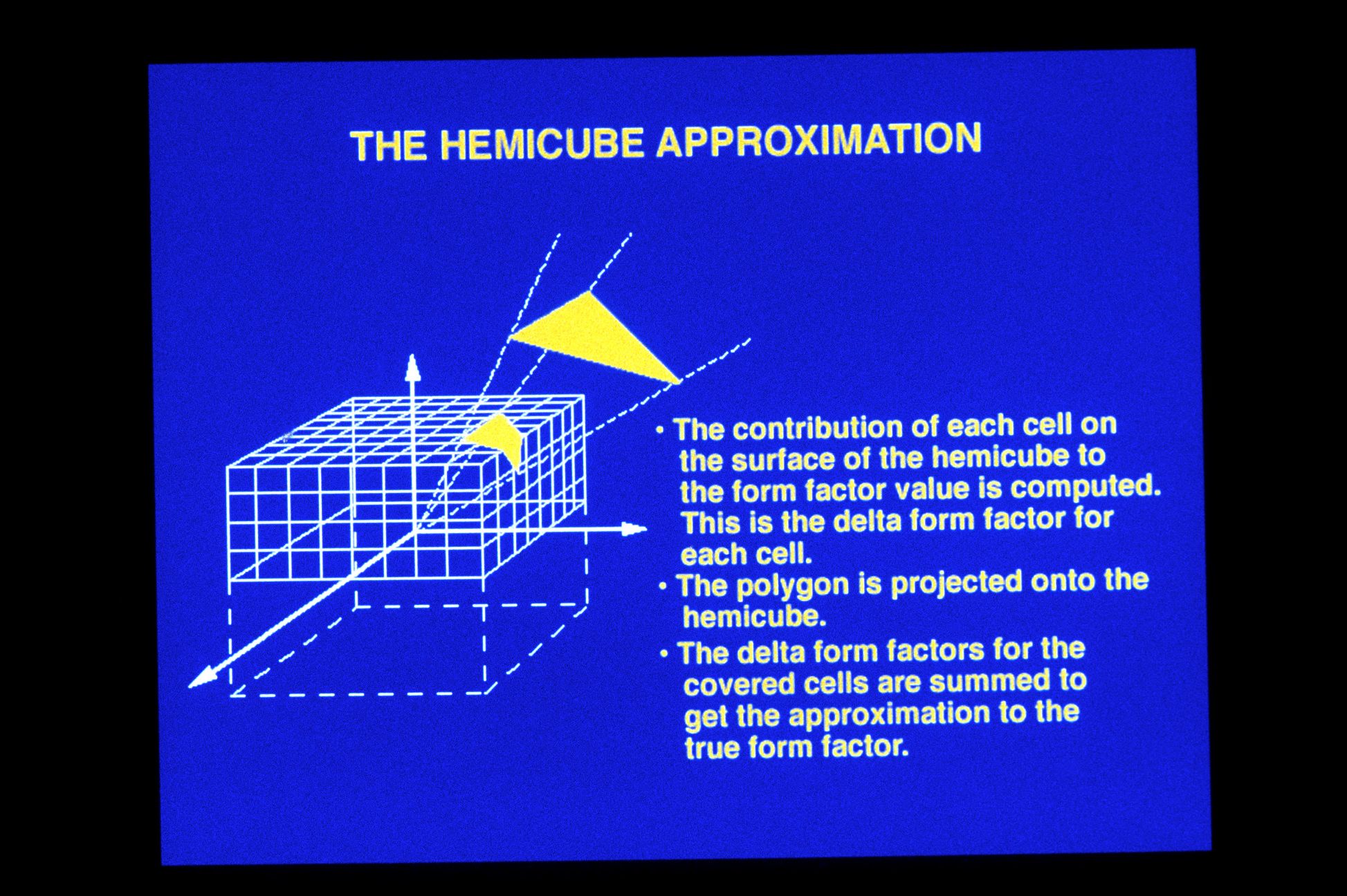
61 – The hemicube
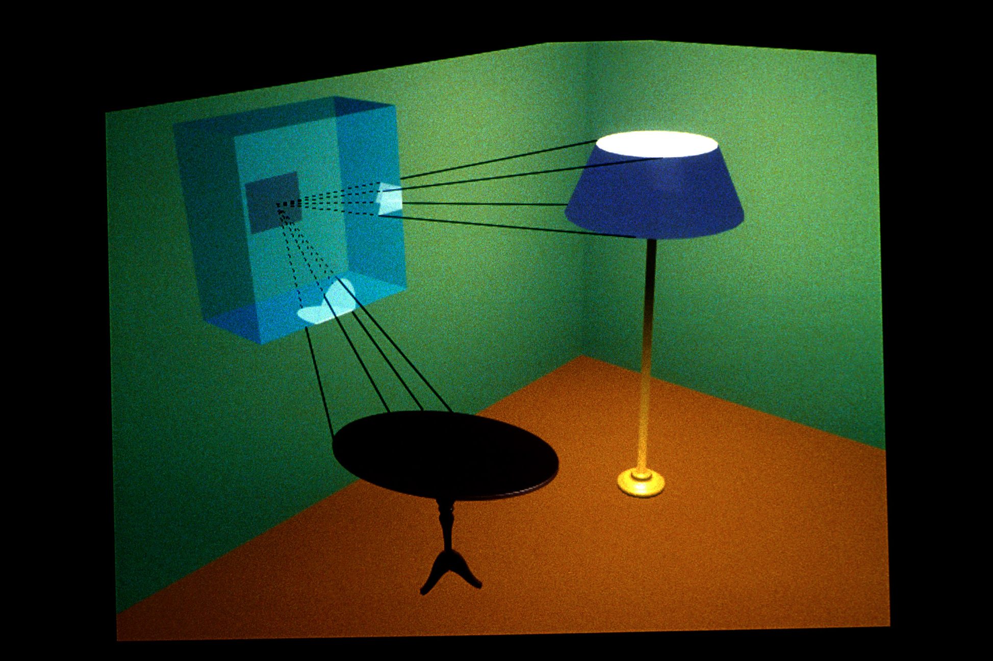
62 – The hemicube in action
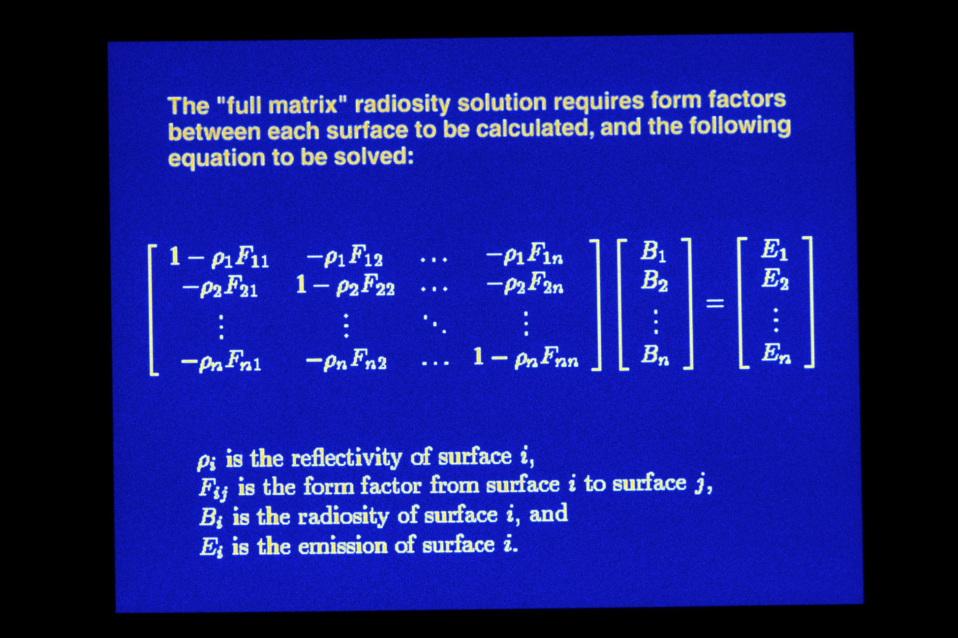
63 – The full matrix radiosity algorithm
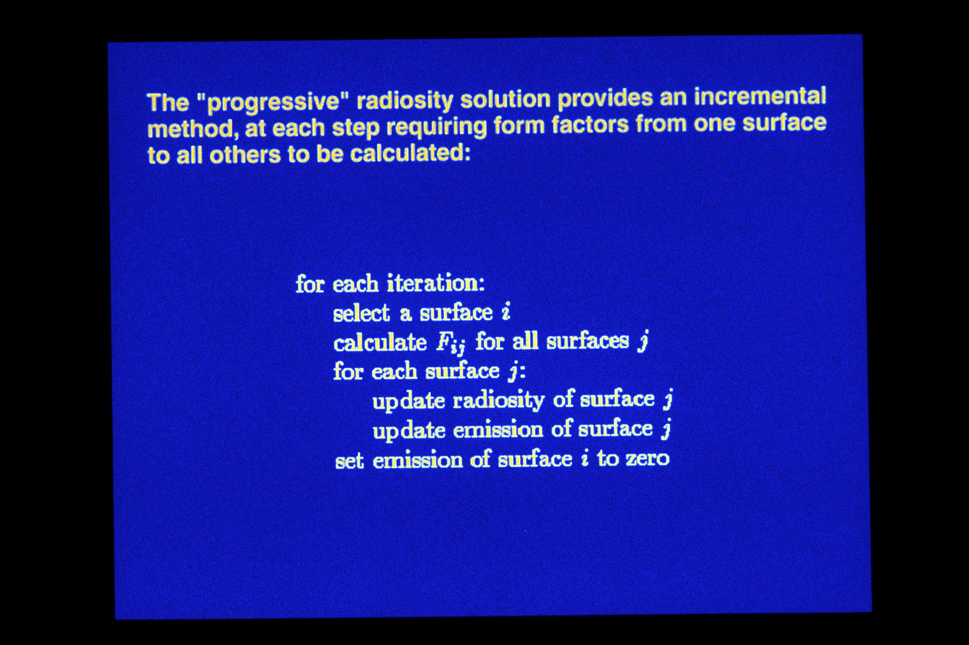
64 – The progressive radiosity algorithm
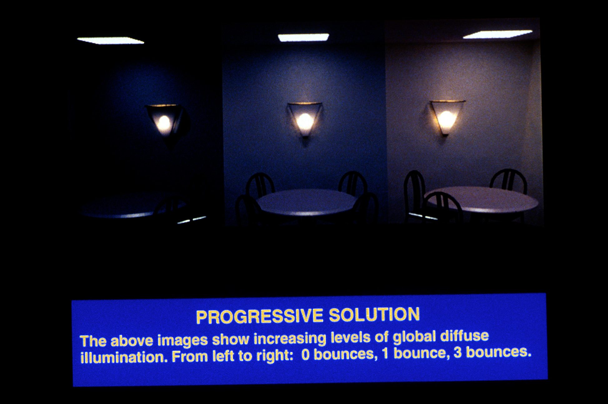
65 – Progressive radiosity examples
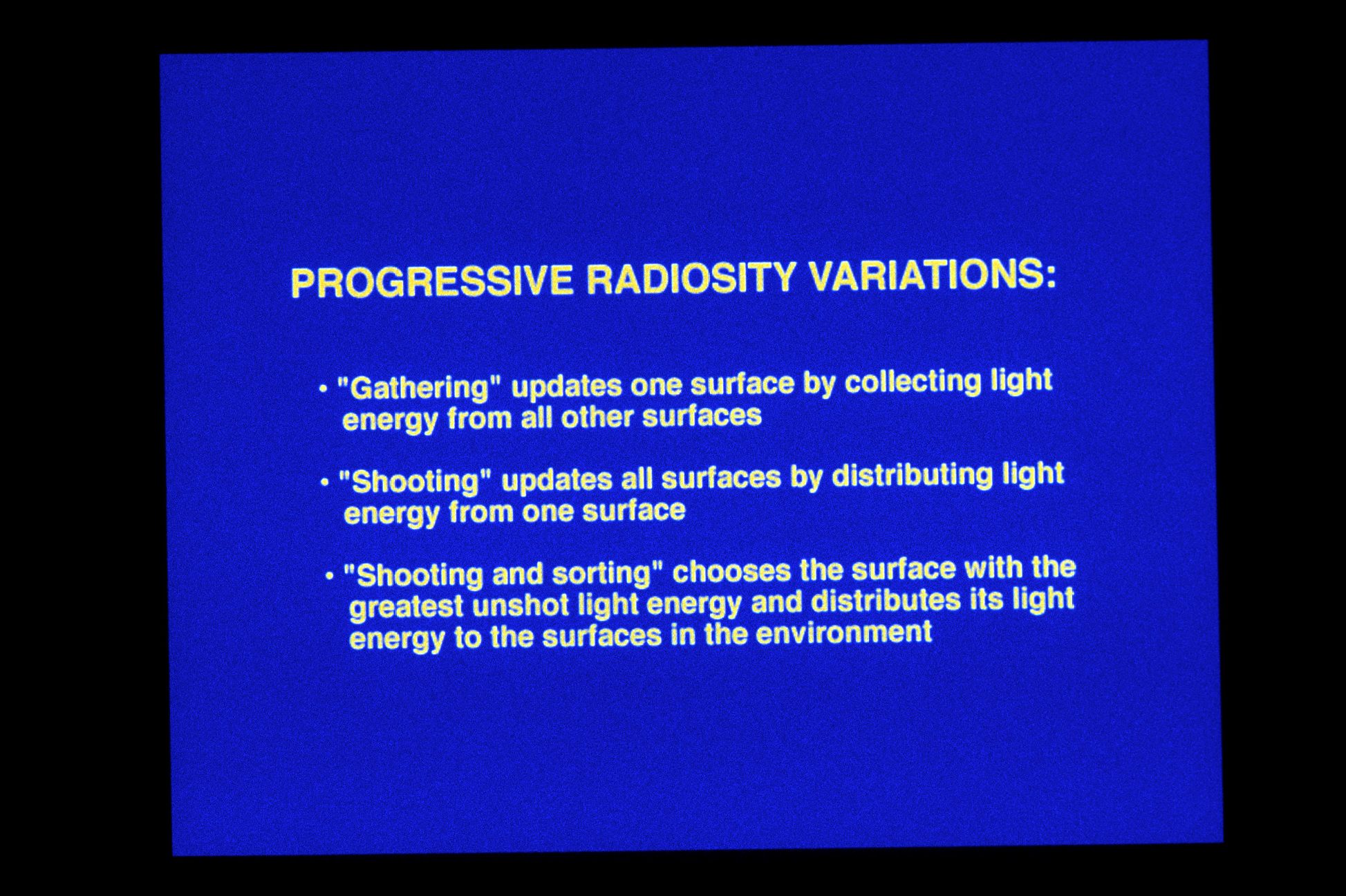
66 – Progressive radiosity variants
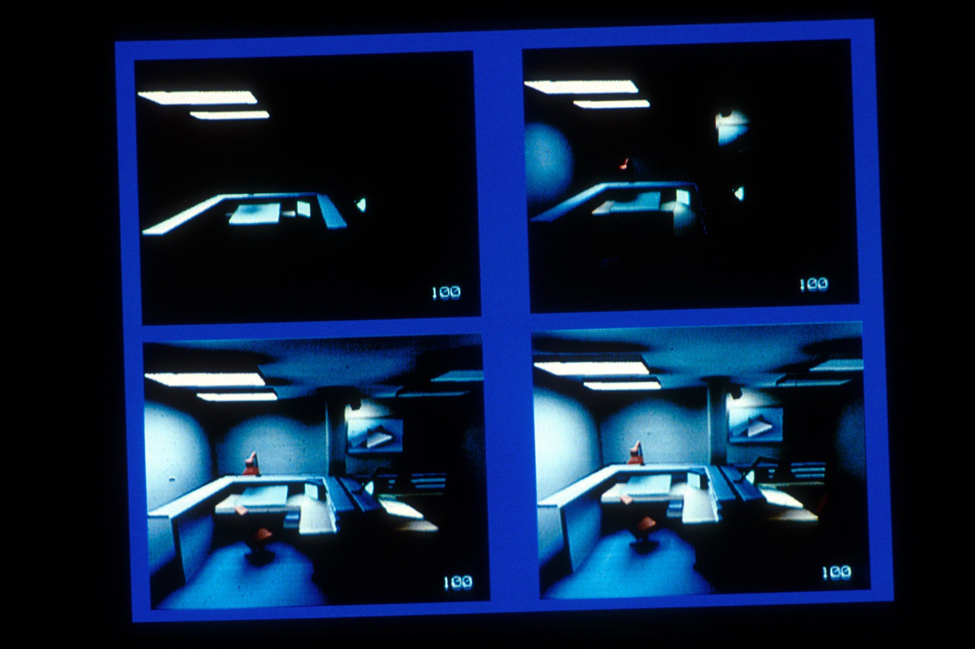
67 – Comparison of progressive variants
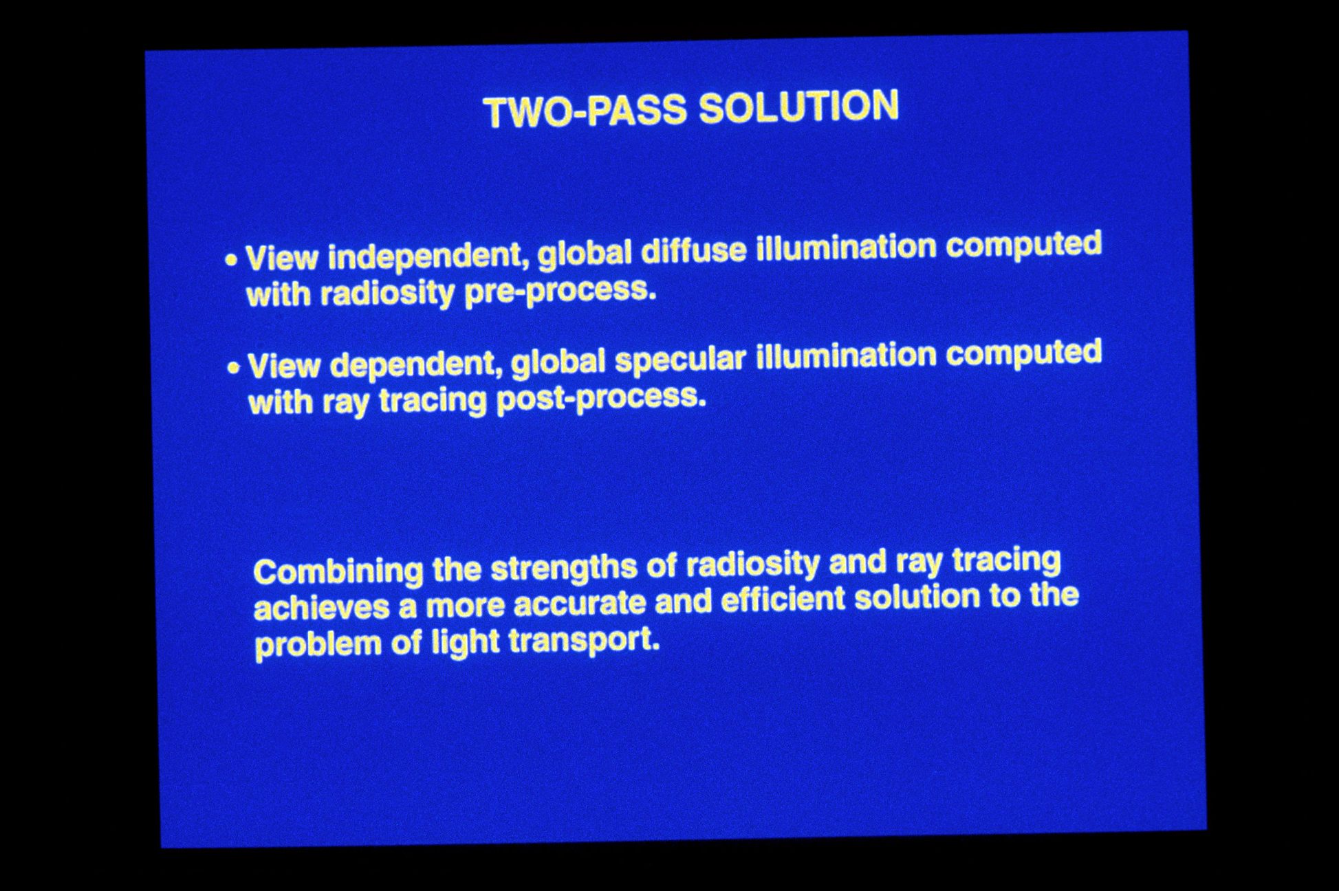
68 – The two-pass radiosity solution
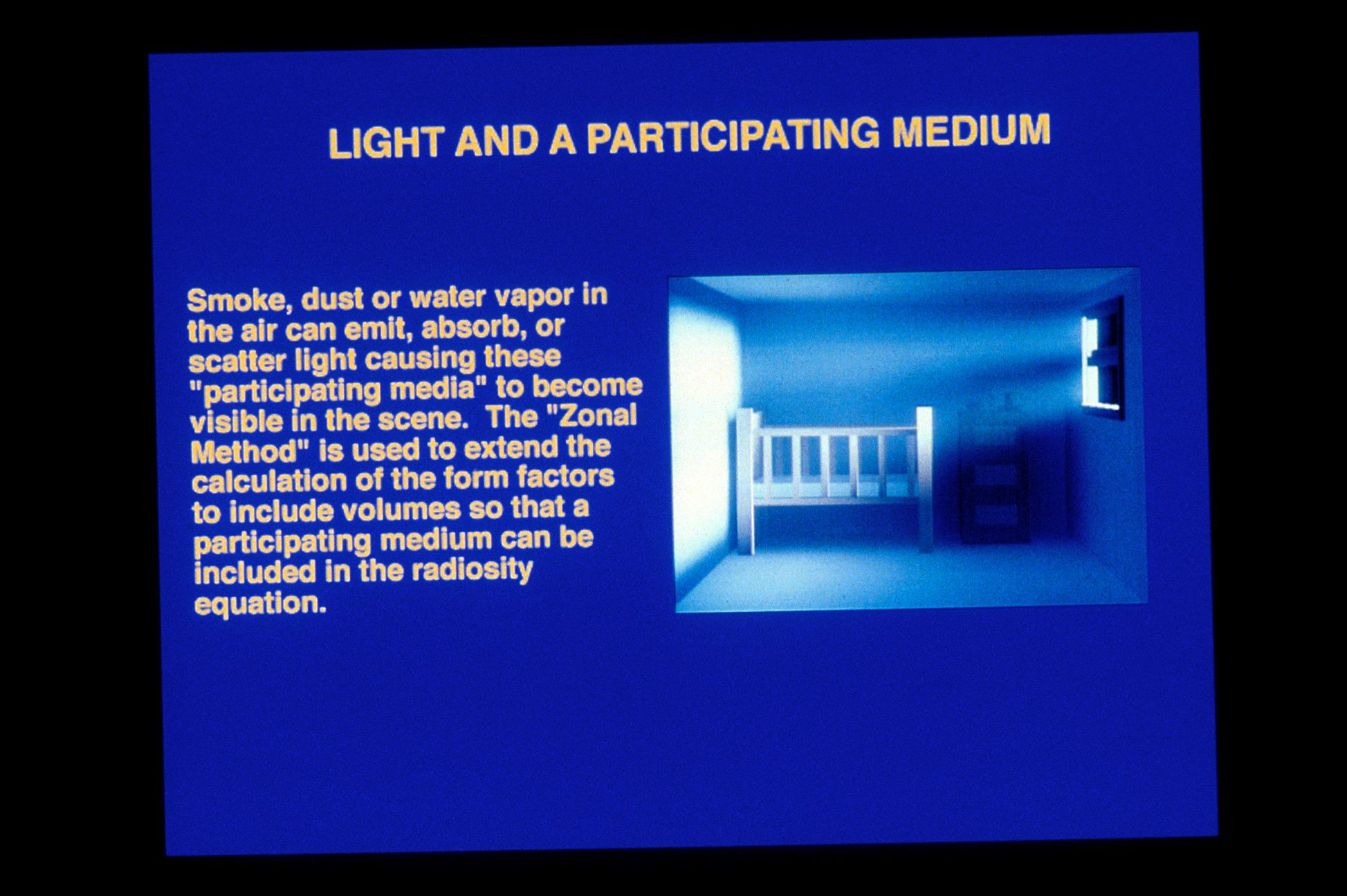
69 – Participating media
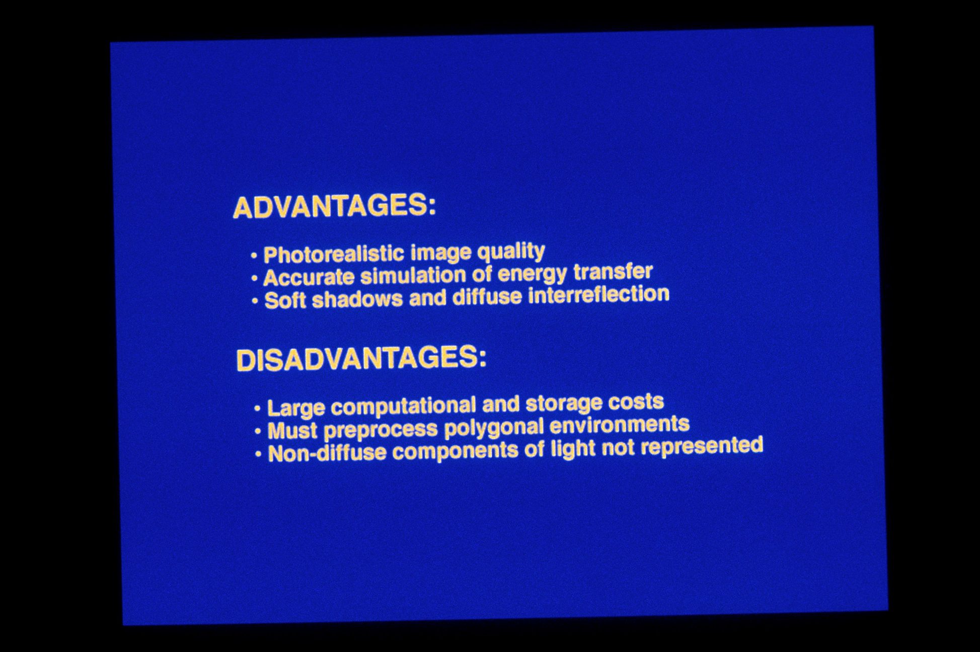
70 – Advantages and disadvantages
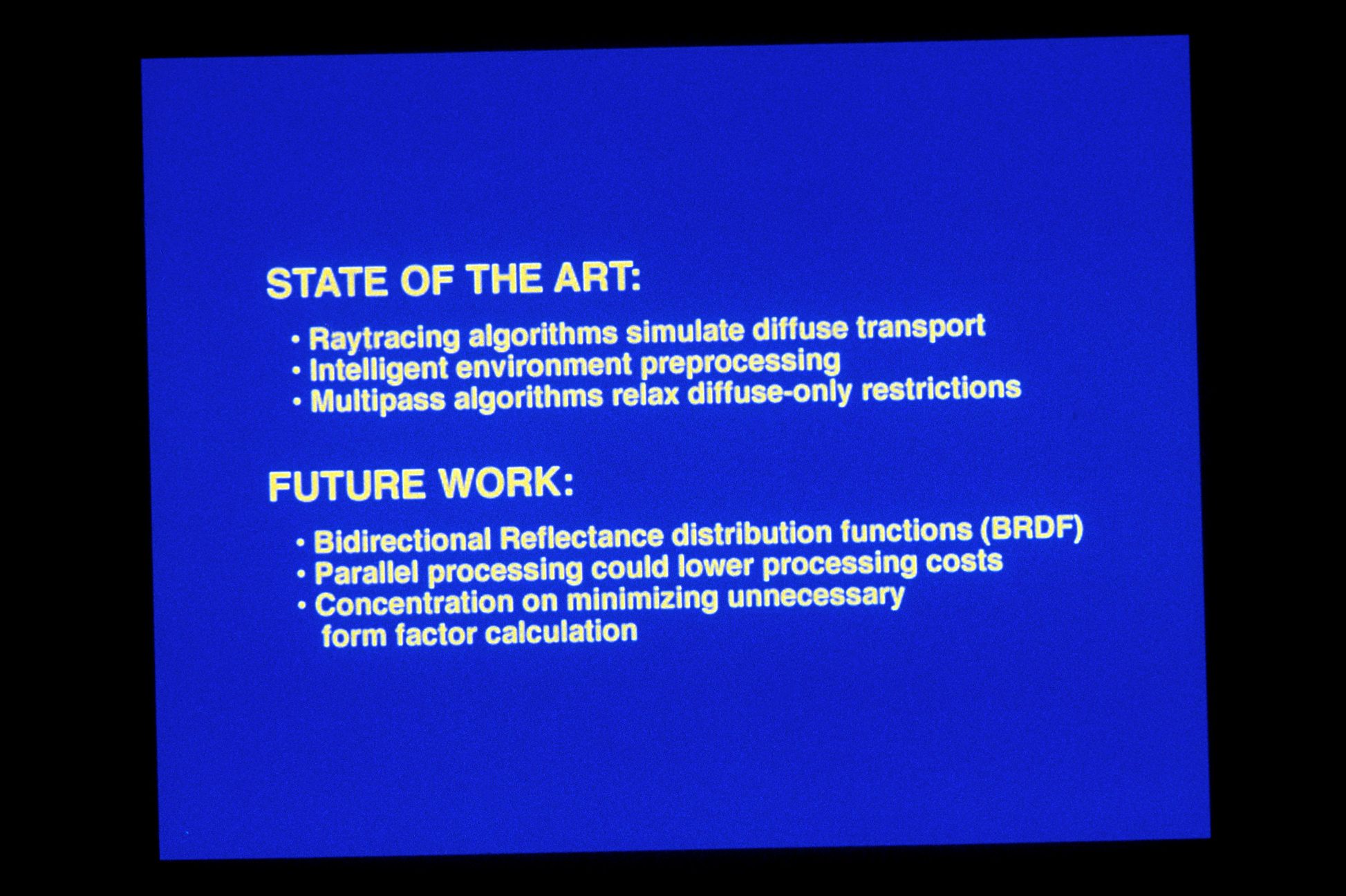
71 – State of the art and future work
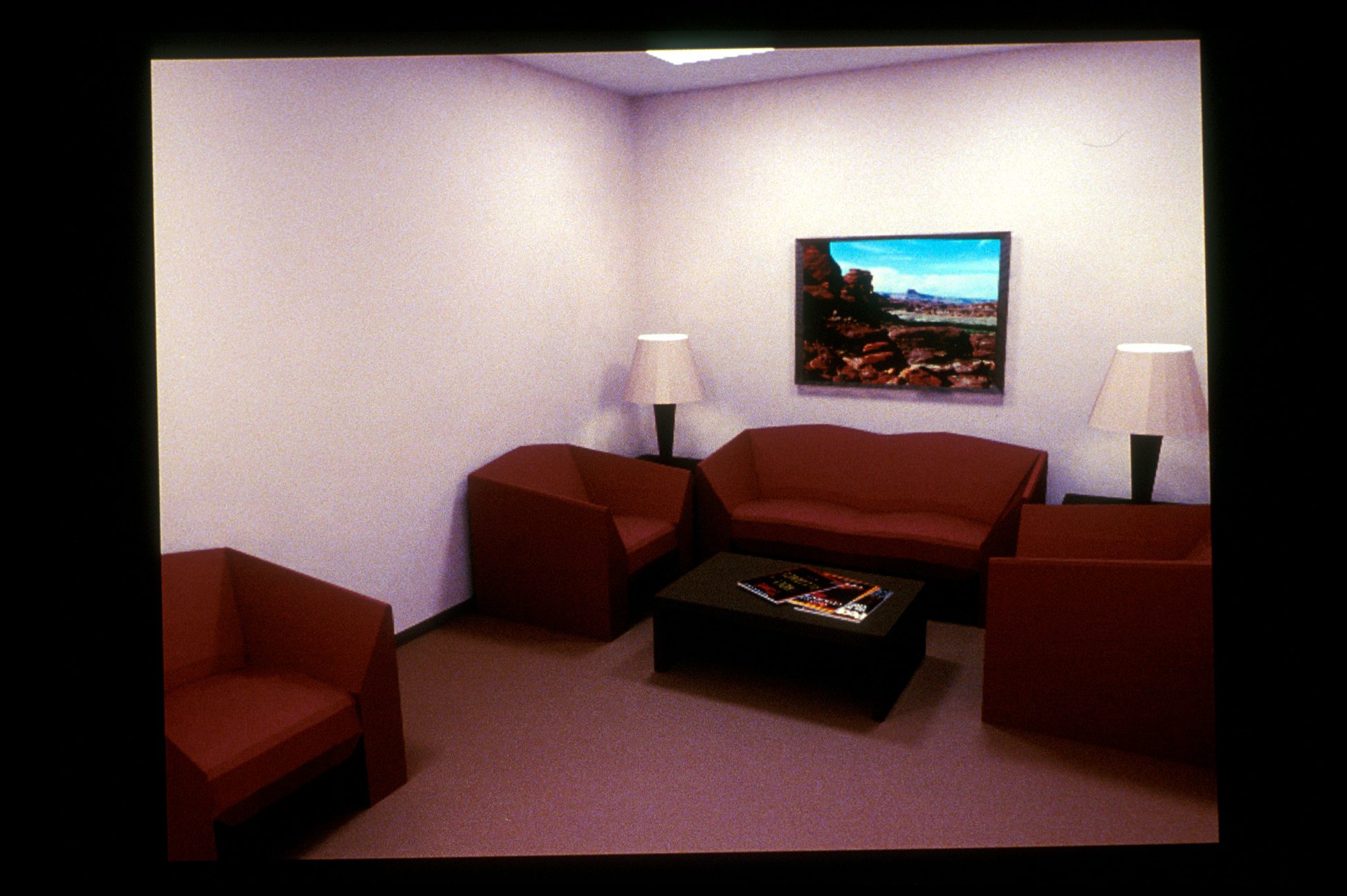
72 – Consolation room image
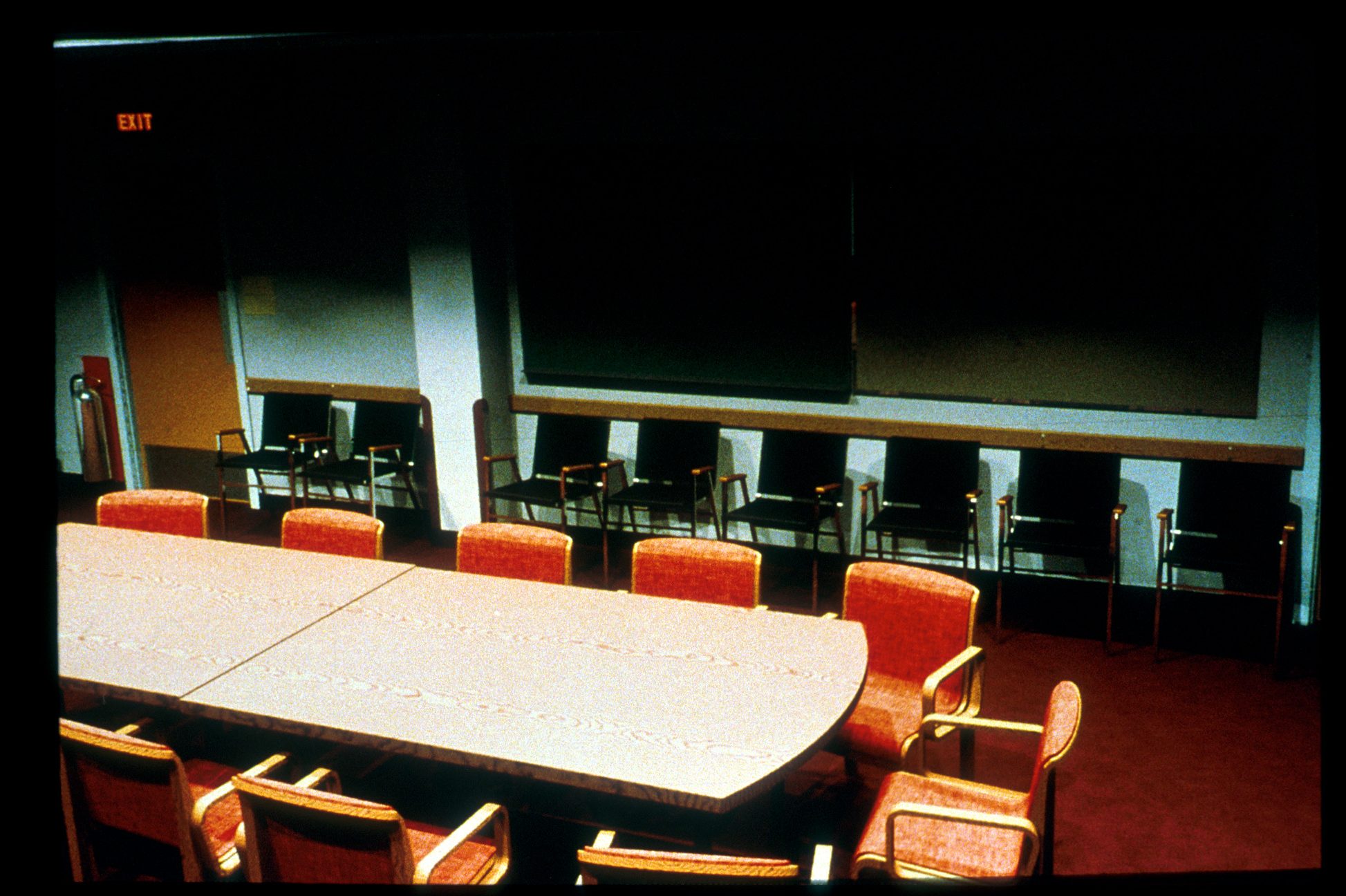
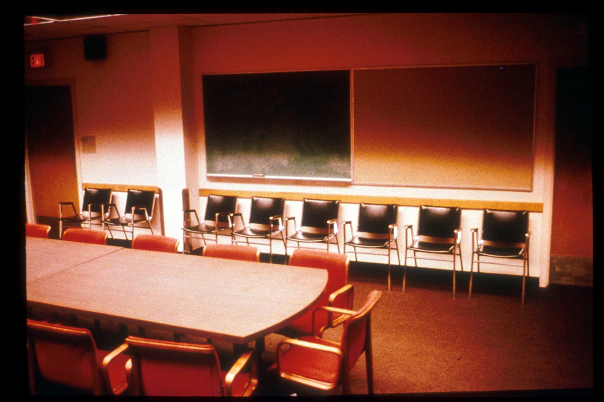
73 – Conference room image
74 – Conference room photograph
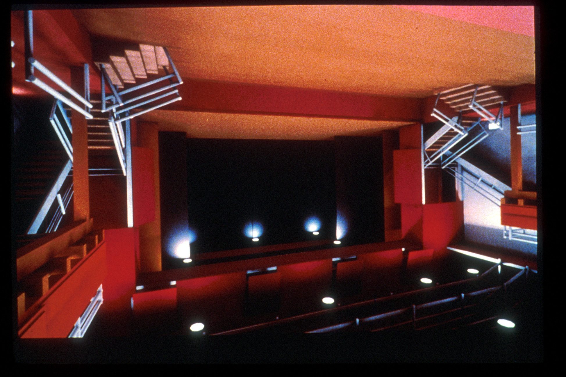
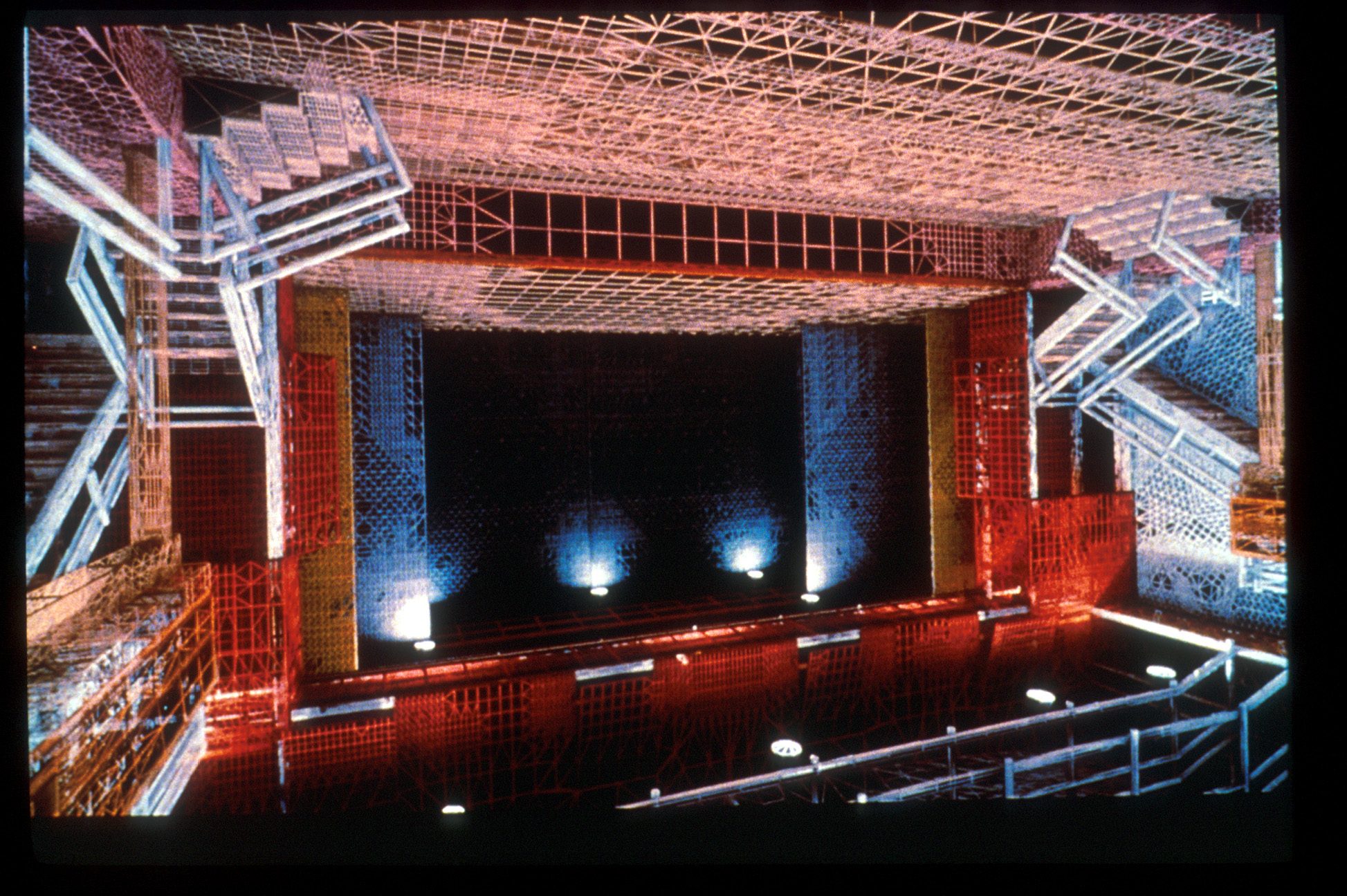
75 – Theatre
76 – Theatre with polygonal mesh
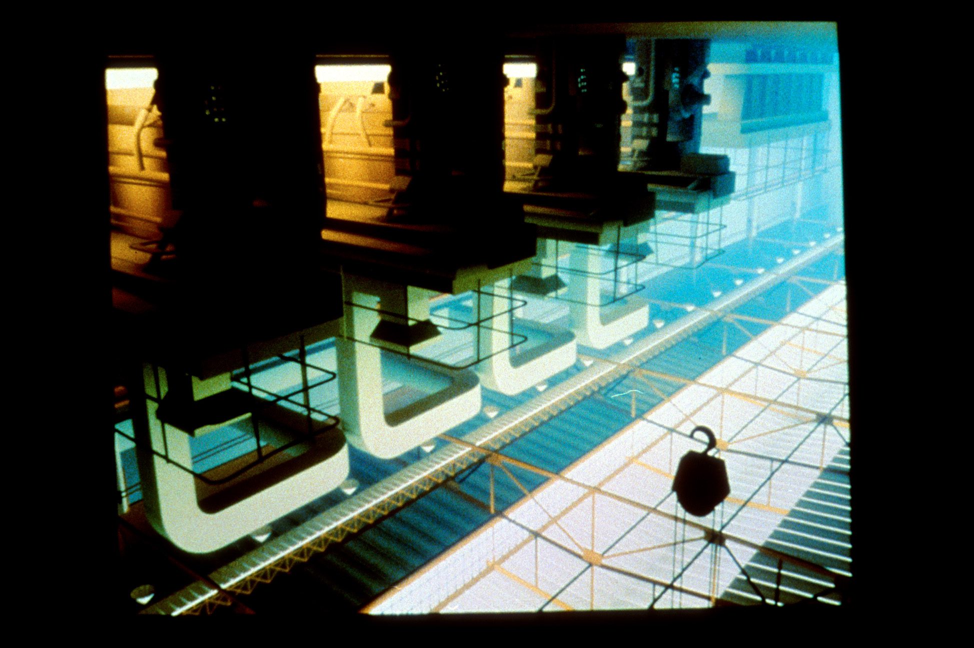
77 – Steel mill
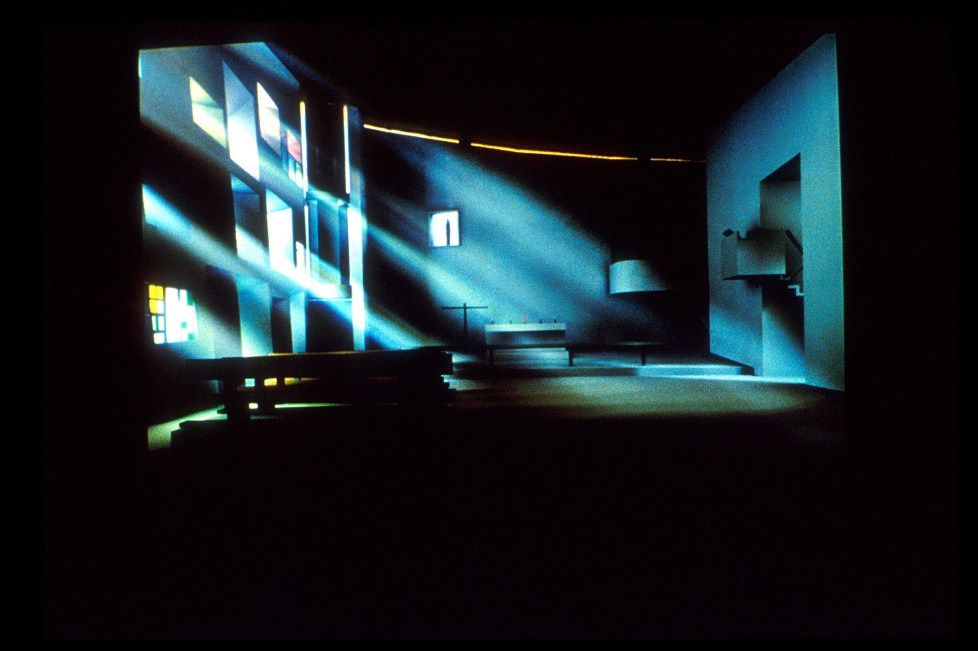
78 – LeCorbusier’s Chapel at Ronchamp
Publication Documents:
1993 Education Slide Set Images: